This topic describes how to use ClickBench and the Star Schema Benchmark (SSB) single-table dataset to perform performance testing on Hologres and ClickHouse and compare the testing results.
ClickBench
ClickBench is the official benchmarking tool for ClickHouse. ClickBench simulates real-world workloads, such as online analytical processing (OLAP) and massive data ingestion, to help users validate database performance, compare efficiency across different configurations or hardware environments, and provide performance tuning references for developers. For more information, see ClickBench.
Test environment
Hologres participated in testing with three instance specifications: 32 CUs, 64 CUs, and 128 CUs. For more information about the testing process, see ClinkBench-Hologres.
Open source ClickHouse, Doris, and StarRocks used
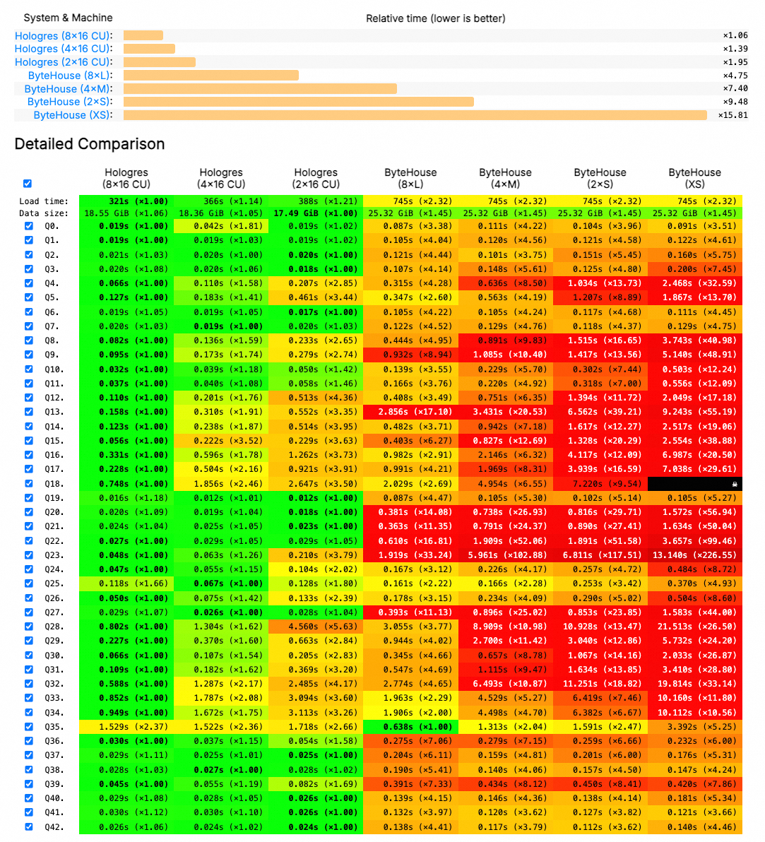
c6a.metalinstances (192 vCPU cores). For more information, see C6a instances.ByteHouse utilized the following computing resource specifications:
8×L: 32 cores
4×M: 16 cores
2×S: 8 cores
XS: 4 cores
Testing result comparison
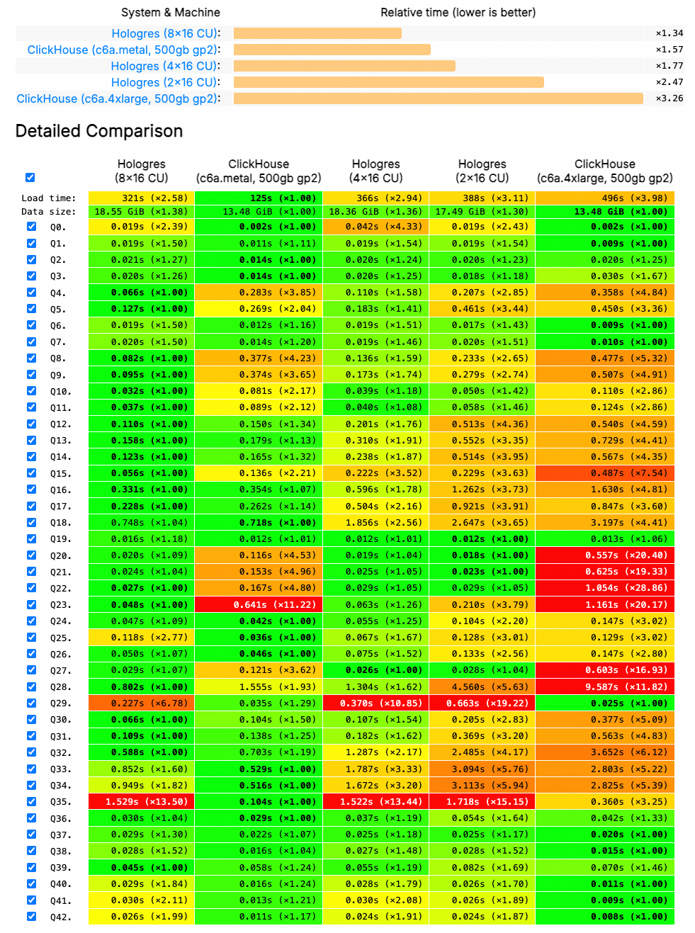
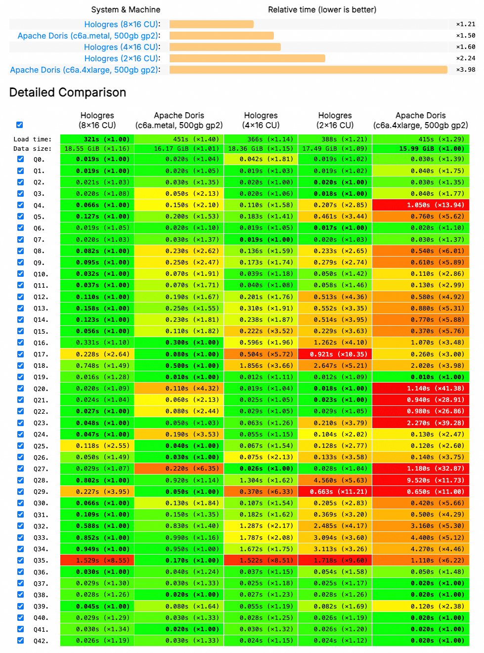
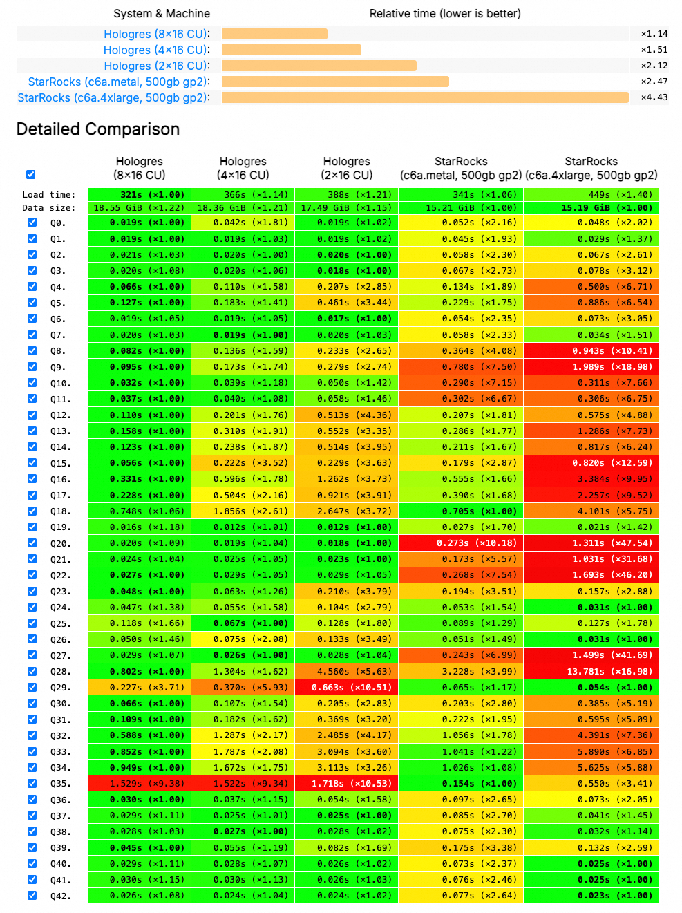
The testing results generated by ClickBench based on the preceding test environment demonstrate that under equivalent computing resources, Hologres exhibits a significant performance advantage over open source alternatives, including ClickHouse, Doris, StarRocks, and ByteHouse. Detailed comparison results are as follows:
Hologres and ClickHouse
Hologres and Doris
Hologres and StarRocks
Hologres and ByteHouse
SSB single-table dataset
Background information
The SSB is a star schema test set widely used in academia and industries. This test set is used to compare the basic performance metrics of various online analytical processing (OLAP) systems. ClickHouse converts the star schema of the SSB to the flat schema and creates a wide table to generate a single-table dataset for testing. For more information, see Star Schema Benchmark on the ClickHouse official website.
This topic describes how to use the single-table dataset based on the SSB to perform performance testing on Hologres and ClickHouse. The following figure shows the test results.
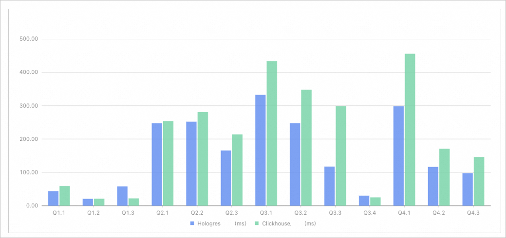
Among the 13 queries on a single table, Hologres is faster than ClickHouse in 11 queries.
In the 13 queries on a single table, the total amount of time used in ClickHouse is 1.35 times that in Hologres.
Test environments
To eliminate the impact of the network bandwidth, this performance testing uses the same Elastic Compute Service (ECS) instance to send query requests to Hologres and ClickHouse in a virtual private cloud (VPC). The result caching feature is disabled in Hologres. The following tables describe the specific test environments.
Test environment in ClickHouse
Item
Description
Server
An ECS instance
CPU
Intel Xeon (Ice Lake) Platinum 8369B, 64 vCPU cores
Memory
256 GiB
Internal bandwidth
32 Gbit/s
Disk
Enhanced SSD (ESSD), 200 GB, PL1, the maximum IOPS of 50,000 per disk
Operating system
CentOS 8.4 64-bit
Hardware fee (excluding the Internet bandwidth)
USD 1370.04 per month
Internet bandwidth over IPv4
200 Mbit/s
Network traffic fee
USD 2323.85 per month
ClickHouse version
V21.8.3.44
Test environment in Hologres
Item
Description
Computing resources
64 CPU cores and 256 GB of memory
Storage resources
Logical storage: 200 GB
Internet bandwidth
Greater than 5 Gbit/s
Total fee
USD 1653.73 per month
Hologres version
V0.10.33
Test data
Table name | Rows of data | Description |
lineorder | 0.6 billion | The commodity order table of the SSB. |
customer | 3 million | The customer table of the SSB. |
part | 1.4 million | The part table of the SSB. |
supplier | 0.2 million | The supplier table of the SSB. |
dates | 2,556 | The date table of the SSB. |
lineorder_flat | 0.6 billion | The wide table of the flat schema based on the tables of the SSB. |
SQL statements
SQL statements in ClickHouse
The DDL statements and query statements used are the same as those provided on the ClickHouse official website. For more information, see Star Schema Benchmark on the ClickHouse official website.
SQL statements in Hologres
DDL statements
DROP TABLE IF EXISTS lineorder_flat;

BEGIN;
CREATE TABLE IF NOT EXISTS lineorder_flat (
  lo_orderdate     date NOT NULL ,
  lo_orderkey      int NOT NULL ,
  lo_linenumber    int NOT NULL ,
  lo_custkey       int NOT NULL ,
  lo_partkey       int NOT NULL ,
  lo_suppkey       int NOT NULL ,
  lo_orderpriority text NOT NULL ,
  lo_shippriority  int NOT NULL ,
  lo_quantity      int NOT NULL ,
  lo_extendedprice int NOT NULL ,
  lo_ordtotalprice int NOT NULL ,
  lo_discount      int NOT NULL ,
  lo_revenue       int NOT NULL ,
  lo_supplycost    int NOT NULL ,
  lo_tax           int NOT NULL ,
  lo_commitdate    date NOT NULL ,
  lo_shipmode      text NOT NULL ,
  c_name           text NOT NULL ,
  c_address text NOT NULL ,
  c_city text NOT NULL ,
  c_nation text NOT NULL ,
  c_region text NOT NULL ,
  c_phone text NOT NULL ,
  c_mktsegment text NOT NULL ,
  s_region text NOT NULL ,
  s_nation text NOT NULL ,
  s_city text NOT NULL ,
  s_name text NOT NULL ,
  s_address text NOT NULL ,
  s_phone text NOT NULL ,
  p_name text NOT NULL ,
  p_mfgr text NOT NULL ,
  p_category text NOT NULL ,
  p_brand text NOT NULL ,
  p_color text NOT NULL ,
  p_type text NOT NULL ,
  p_size int NOT NULL ,
  p_container text NOT NULL,
  PRIMARY KEY (lo_orderkey,lo_linenumber)
);
CALL set_table_property('lineorder_flat', 'distribution_key', 'lo_orderkey');
CALL set_table_property('lineorder_flat', 'segment_key', 'lo_orderdate');
CALL set_table_property('lineorder_flat', 'clustering_key', 'lo_orderdate');
CALL set_table_property('lineorder_flat', 'bitmap_columns', 'p_category,s_region,c_region,c_nation,s_nation,c_city,s_city,p_mfgr,p_brand');
CALL set_table_property('lineorder_flat', 'time_to_live_in_seconds', '31536000');
COMMIT;
Query statements
Q1.1
SELECT SUM(LO_EXTENDEDPRICE * LO_DISCOUNT) AS REVENUE
FROM LINEORDER_FLAT
WHERE LO_ORDERDATE >= DATE '1993-01-01'
AND LO_ORDERDATE <= DATE '1993-12-31'
AND LO_DISCOUNT BETWEEN 1 AND 3
AND LO_QUANTITY < 25;
Q1.2
SELECT SUM(LO_EXTENDEDPRICE * LO_DISCOUNT) AS REVENUE
FROM LINEORDER_FLAT
WHERE LO_ORDERDATE >= DATE '1994-01-01'
AND LO_ORDERDATE <= DATE '1994-01-31'
AND LO_DISCOUNT BETWEEN 4 AND 6
AND LO_QUANTITY BETWEEN 26 AND 35;
Q1.3
SELECT SUM(LO_EXTENDEDPRICE * LO_DISCOUNT) AS REVENUE
FROM LINEORDER_FLAT
WHERE EXTRACT(WEEK FROM LO_ORDERDATE ) = 6
AND LO_ORDERDATE >= DATE '1994-01-01'
AND LO_ORDERDATE <= DATE '1994-12-31'
AND LO_DISCOUNT BETWEEN 5 AND 7
AND LO_QUANTITY BETWEEN 26 AND 35;
Q2.1
SELECT SUM(LO_REVENUE),
EXTRACT(YEAR FROM LO_ORDERDATE) AS YEAR,
P_BRAND
FROM LINEORDER_FLAT
WHERE P_CATEGORY = 'MFGR#12'
AND S_REGION = 'AMERICA'
GROUP BY YEAR, P_BRAND
ORDER BY YEAR, P_BRAND;
Q2.2
SELECT SUM(LO_REVENUE),
EXTRACT(YEAR FROM LO_ORDERDATE) AS YEAR,
P_BRAND
FROM LINEORDER_FLAT
WHERE P_BRAND BETWEEN 'MFGR#2221' AND 'MFGR#2228'
AND S_REGION = 'ASIA'
GROUP BY YEAR, P_BRAND
ORDER BY YEAR, P_BRAND;
Q2.3
SELECT SUM(LO_REVENUE),
EXTRACT(YEAR FROM LO_ORDERDATE) AS YEAR,
P_BRAND
FROM LINEORDER_FLAT
WHERE P_BRAND = 'MFGR#2239'
AND S_REGION = 'EUROPE'
GROUP BY YEAR, P_BRAND
ORDER BY YEAR, P_BRAND;
Q3.1
SELECT C_NATION,
S_NATION,
EXTRACT(YEAR FROM LO_ORDERDATE) AS YEAR,
SUM(LO_REVENUE) AS REVENUE
FROM LINEORDER_FLAT
WHERE C_REGION = 'ASIA'
AND S_REGION = 'ASIA'
AND LO_ORDERDATE  >= DATE '1992-01-01'
AND LO_ORDERDATE  <= DATE '1997-12-31'
GROUP BY C_NATION,S_NATION,YEAR
ORDER BY  YEAR ASC,REVENUE DESC;
Q3.2
SELECT C_CITY,
S_CITY,
EXTRACT(YEAR FROM LO_ORDERDATE) AS YEAR,
SUM(LO_REVENUE) AS REVENUE
FROM LINEORDER_FLAT
WHERE C_NATION = 'UNITED STATES'
AND S_NATION = 'UNITED STATES'
AND LO_ORDERDATE >= DATE '1992-01-01'
AND LO_ORDERDATE <= DATE '1997-12-31'
GROUP BY C_CITY, S_CITY, YEAR
ORDER BY YEAR ASC, REVENUE DESC;
Q3.3
SELECT C_CITY,
S_CITY,
EXTRACT(YEAR FROM LO_ORDERDATE) AS YEAR,
SUM(LO_REVENUE) AS REVENUE
FROM LINEORDER_FLAT
WHERE C_CITY IN ( 'UNITED KI1' ,'UNITED KI5')
AND S_CITY IN ( 'UNITED KI1' ,'UNITED KI5')
AND LO_ORDERDATE >= DATE '1992-01-01'
AND LO_ORDERDATE <= DATE '1997-12-31'
GROUP BY C_CITY, S_CITY, YEAR
ORDER BY YEAR ASC, REVENUE DESC;
Q3.4
SELECT C_CITY,
S_CITY,
EXTRACT(YEAR FROM LO_ORDERDATE) AS YEAR,
SUM(LO_REVENUE) AS REVENUE
FROM LINEORDER_FLAT
WHERE C_CITY IN ('UNITED KI1', 'UNITED KI5')
AND S_CITY IN ( 'UNITED KI1',  'UNITED KI5')
AND LO_ORDERDATE >= DATE '1997-12-01'
AND LO_ORDERDATE <= DATE '1997-12-31'
GROUP BY C_CITY, S_CITY, YEAR
ORDER BY YEAR ASC, REVENUE DESC;
Q4.1
SELECT EXTRACT(YEAR FROM LO_ORDERDATE) AS YEAR,
C_NATION,
SUM(LO_REVENUE - LO_SUPPLYCOST) AS PROFIT
FROM LINEORDER_FLAT
WHERE C_REGION = 'AMERICA'
AND S_REGION = 'AMERICA'
AND P_MFGR IN ( 'MFGR#1' , 'MFGR#2')
GROUP BY YEAR, C_NATION
ORDER BY YEAR ASC, C_NATION ASC;
Q4.2
SELECT EXTRACT(YEAR FROM LO_ORDERDATE) AS YEAR,
S_NATION,
P_CATEGORY,
SUM(LO_REVENUE - LO_SUPPLYCOST) AS PROFIT
FROM LINEORDER_FLAT
WHERE C_REGION = 'AMERICA'
AND S_REGION = 'AMERICA'
AND LO_ORDERDATE >= DATE '1997-01-01'
AND LO_ORDERDATE <= DATE '1998-12-31'
AND  P_MFGR IN ( 'MFGR#1' , 'MFGR#2')
GROUP BY YEAR, S_NATION, P_CATEGORY
ORDER BY  YEAR ASC, S_NATION ASC, P_CATEGORY ASC;
Q4.3
SELECT EXTRACT(YEAR FROM LO_ORDERDATE) AS YEAR,
S_CITY,
P_BRAND,
SUM(LO_REVENUE - LO_SUPPLYCOST) AS PROFIT
FROM LINEORDER_FLAT
WHERE S_NATION = 'UNITED STATES'
AND LO_ORDERDATE >= DATE '1997-01-01'
AND LO_ORDERDATE <= DATE '1998-12-31'
AND P_CATEGORY = 'MFGR#14'
GROUP BY  YEAR,  S_CITY, P_BRAND
ORDER BY YEAR ASC,  S_CITY ASC,  P_BRAND ASC;
Test results
Query statement | Amount of time used in Hologres (Unit: ms) | Amount of time used in ClickHouse (Unit: ms) | Amount of time used in ClickHouse/Amount of time used in Hologres (Unit: times) |
Q1.1 | 43.66 | 59.00 | 1.35 |
Q1.2 | 20.68 | 21.00 | 1.02 |
Q1.3 | 57.98 | 22.00 | 0.38 |
Q2.1 | 247.63 | 254.00 | 1.03 |
Q2.2 | 251.90 | 281.00 | 1.12 |
Q2.3 | 165.73 | 214.00 | 1.29 |
Q3.1 | 332.84 | 434.00 | 1.30 |
Q3.2 | 247.79 | 348.00 | 1.40 |
Q3.3 | 117.46 | 299.00 | 2.55 |
Q3.4 | 30.05 | 25.00 | 0.83 |
Q4.1 | 298.48 | 456.00 | 1.53 |
Q4.2 | 116.47 | 171.00 | 1.47 |
Q4.3 | 97.68 | 146.00 | 1.49 |
Total | 2,028.35 | 2,730.00 | 1.35 |