Hologres integrates stream and batch processing with Flink, MaxCompute, and DataWorks to support real-time data warehouse architectures. This guide covers three layering approaches—ad hoc queries, near real-time processing, and incremental computing—to help you choose the right design for your latency, throughput, and development efficiency requirements.
Background
Traditional data warehouse development processes data through sequential layers: Operational Data Store (ODS) > Data Warehouse Detail (DWD) > Data Warehouse Summary (DWS) > Application Data Service (ADS). Tasks are scheduled between layers in an event-driven or micro-batch manner. This approach provides semantic abstraction and data reuse, but also introduces scheduling dependencies, increases latency, and reduces analysis agility.
Real-time data warehouses change that dynamic. Business decisions now require rich, contextual data—which strains the traditional model of maintaining thousands of ADS tables, each customized for a specific business unit. More teams want to run multi-dimensional analysis directly at the DWS or DWD layer, placing higher demands on query engine performance, scheduling efficiency, and I/O throughput.
Hologres addresses this through query engine technologies such as vectorized operator rewrites, fine-grained indexing, asynchronous execution, and tiered caching. As a result, many teams adopt a leaner approach: clean data and perform large table joins at the DWD layer, stop modeling there or at DWS, and rely on Hologres's interactive query engine for flexible analysis—achieving responses in seconds.
The following three approaches let you balance agility, latency, and resource cost.
Choose a scenario
| Scenario 1: Ad hoc queries | Scenario 2: Near real-time | Scenario 3: Incremental computing | |
|---|---|---|---|
| Latency | Low (immediate after write) | Minute-level | Lowest |
| QPS support | Low to medium | High | Low to medium |
| Development complexity | Low | Medium | High (requires advanced Flink skills) |
| Compute cost | Medium | Medium | High |
| Best for | Flexible ad hoc analysis, low query complexity, sufficient resources | Most real-time analytics workloads (over 80% of use cases) | Latency-critical online services |
Scenario 1 is the right choice when:
Queries must reflect data immediately after it is written
Analysis patterns are not predetermined and flexibility is essential
Query complexity is low and compute resources are sufficient
Queries per second (QPS) requirements are moderate
Scenario 2 is the right choice when:
Both QPS and near real-time freshness are required
Your team prioritizes development efficiency over sub-minute latency
Minute-level latency (for example, 5 or 10 minutes) is acceptable
Scenario 3 is the right choice when:
Data latency requirements are stricter than Scenario 2 can provide (for example, latency must stay under a few seconds end to end)
Data updates are infrequent and results can be computed cumulatively from incremental data
The workload is primarily simple statistics on instrumentation data for online services such as dashboards and risk control
Your team has advanced Flink expertise
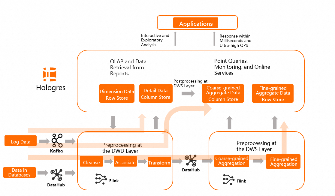
Scenario 1: Ad hoc queries
Best for: Teams that need maximum flexibility and have not yet defined fixed query patterns. Query complexity must be low and compute resources must be sufficient to handle complex view queries at runtime.
In this approach, raw data is stored at the detail layer first. All aggregation and business logic is deferred to query time through views, so you can adjust the logic without touching underlying tables.

Architecture:
Clean and join ODS layer data. Store the results as detail data without further aggregation. Write the detail data directly to Hologres.
Use Flink to process incremental data and update the detail data in Hologres in real time. Write offline tables processed by MaxCompute to Hologres.
At the Common Data Model (CDM) or ADS layer, encapsulate business logic as views rather than physical tables. Views defer all aggregation to query time, keeping the upper layers flexible and easy to correct.
Upper-layer applications query the views directly for ad hoc analysis.
Advantages:
High flexibility. Adjust views at any time as business logic evolves, without modifying underlying tables.
Easy metric correction. Because no aggregation tables exist in the upper layers, fixing a data issue only requires updating the underlying detail tables.
Disadvantage: Query performance degrades when view logic is complex and data volumes are large. This becomes a problem when QPS requirements increase or when multiple upstream joins are nested in views. If your workload starts requiring higher QPS or sub-minute latency, move to Scenario 2.
Typical data sources: Databases and instrumentation systems.
Scenario 2: Near real-time at the minute level
Best for: Teams that need both high QPS and near real-time data freshness, and can accept minute-level latency. This covers over 80% of real-time data warehouse use cases.
Scenario 2 extends Scenario 1 by materializing views into physical tables at the CDM and ADS layers. The aggregated tables contain far less data than the underlying detail tables, which significantly improves query performance and allows for higher QPS.
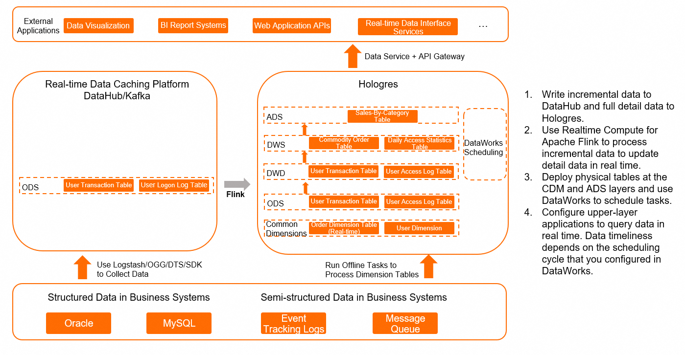
Architecture:
Clean and join ODS layer data. Store the results as detail data without further aggregation. Write the detail data directly to Hologres.
Use Flink to process incremental data and update the detail data in Hologres in real time.
At the CDM and ADS layers, use physical tables instead of views. Use DataWorks to schedule periodic writes on a 5-minute or 10-minute cycle.
Upper-layer applications query the physical tables directly. Data freshness depends on the DataWorks scheduling cycle.
Why physical tables instead of views? At this scale, views recompute aggregations on every query. Physical tables pre-compute the aggregations and store only the result set, reducing the data volume each query must scan and enabling higher QPS.
Advantages:
High query performance. Applications query pre-aggregated data rather than raw detail tables.
Fast data refresh. If a step fails or data is incorrect, rerun the DataWorks scheduling task. Because all logic is expressed in SQL, no complex correction procedures are needed.
Fast business logic adjustment. Add or modify business logic at any layer using SQL in a What You See Is What You Get (WYSIWYG) manner, shortening the go-live cycle.
Disadvantage: Latency is higher than Scenario 1 because data must pass through a DataWorks scheduling cycle before becoming available. This is a problem if your business requires data to be queryable within seconds of generation.
When to move to Scenario 3: If a 5–10 minute scheduling cycle is still too long—for example, for risk control or real-time dashboards where decisions must reflect the latest incremental data within seconds, and your team has strong Flink expertise with infrequently updated data—consider Scenario 3.
Typical data sources: Databases and instrumentation systems.
Scenario 3: Real-time statistics for incremental data
Best for: Teams with strict latency requirements (stricter than minute-level), simple real-time needs based on instrumentation data, and strong Flink expertise.
In this approach, Flink handles all pre-aggregation before data reaches Hologres. Hologres stores only the final result sets and serves them directly to upper-layer applications.
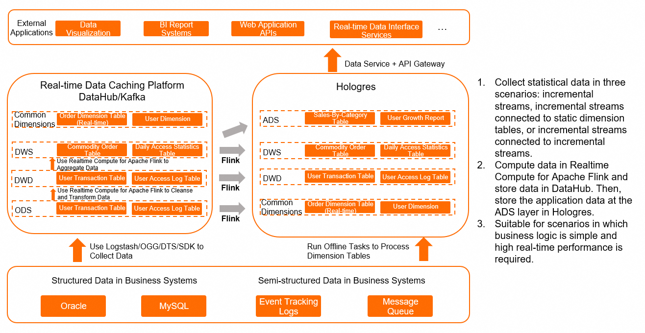
Architecture:
Use Flink to clean, transform, and aggregate the data for incremental computing. Store the application data from the ADS layer in Hologres.
Write Flink result sets in dual-write mode: deliver results to the message stream topic of the next layer, and simultaneously sink them to Hologres at the same layer. This preserves intermediate states for status checks and historical data refreshes.
Within Flink, gather statistics using one of three methods: using an incremental stream, joining an incremental stream with a static dimension table, or joining two incremental streams.
Hologres serves the result tables directly to upper-layer applications for real-time queries.
Why dual-write mode? Writing intermediate states to both the message stream and Hologres makes it easier to inspect and correct data if quality issues arise, without having to reprocess the entire pipeline.
Advantages:
Lowest latency. Data is available for query as soon as Flink processes each event.
Easy metric correction. Unlike traditional incremental computing, intermediate states are persisted in Hologres. If data quality issues appear in intermediate data, correct the table directly and refresh from there.
Disadvantages:
High Flink dependency. Most aggregation logic runs in Flink, which requires advanced proficiency. This becomes a problem if the team is not experienced with stateful stream processing.
Limited to cumulative computations. This approach does not work for scenarios with frequent data updates that cannot be cumulatively calculated, or for computationally intensive scenarios such as multi-stream joins.
Typical data sources: Instrumentation systems with small data volumes and simple real-time statistics requirements.