By Daoke
In PolarDB for MySQL 8.0.1, the parallel query is a relatively simple two-phase execution model (scatter-gather model) and subject to the following limits:
• The simple execution framework may lead to single-point bottlenecks for some heavily used computing operators (grouping and aggregation).
• Operator parallelism is not fully supported. For example, window functions and nested derived tables do not support parallelism.
• The parallel execution of operators is simple. For example, all joins must be pushed down. Group aggregation is executed in two phases.
These limits make parallel query 1.0 not ideal for complex analytic queries.
In PolarDB for MySQL 8.0.2, parallel query is upgraded to version 2.0, which solves the limits mentioned above and provides comprehensive support for complex analytic queries.
• A multi-phase execution framework can parse SQL statements into multiple computing operators. Each operator can be distributed to multiple workers for parallel execution. The operators in a worker are efficiently executed in a pipelined manner.
• Parallelism of all operators is supported.
• Diverse operator parallelism methods are supported, such as shuffle join, one-phase group aggregation, and cost-based parallelism selection.
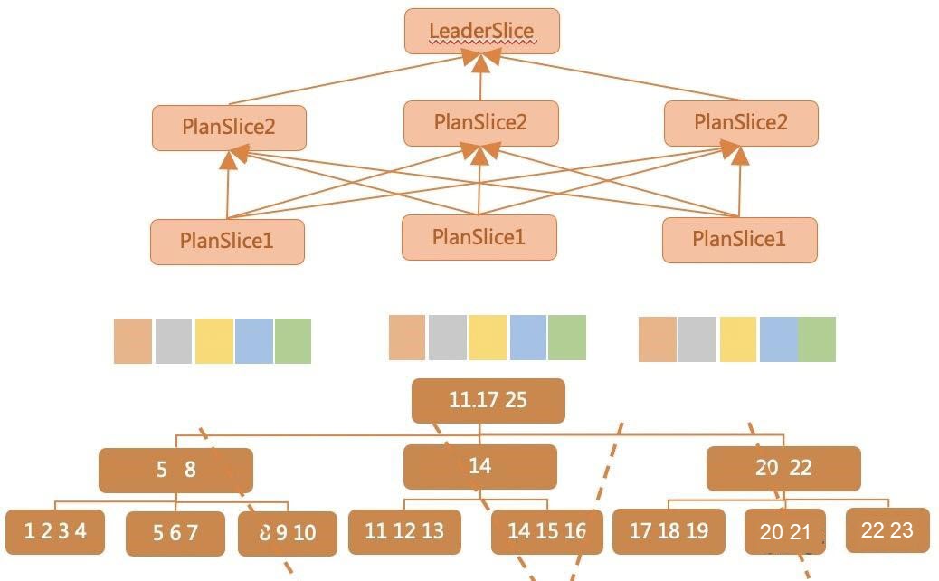
Example:
SQL:
SELECT t1.a, sum(t2.b) sumb, count(t3.c) countc
FROM
t1 JOIN t2 on t1.a = t2.a JOIN t3 on t2.b = t3.b
GROUP BY t1.a
ORDER BY sumb;
Improvement of parallel planning:
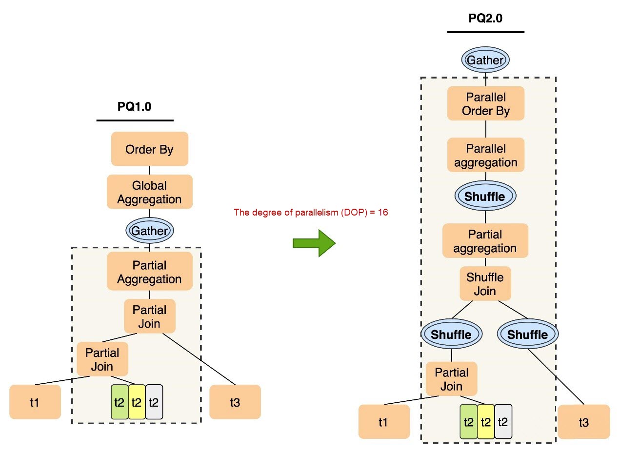
On the left side of the figure is the parallel plan generated by parallel query 1.0. Two problems can be seen.
On the right side of the figure is the parallel plan that parallel query 2.0 produces, which solves the two problems by the following means:
TPC BenchmarkH (TPC-H) provides 22 SQL queries. In the following example, the eleventh SQL query is used.
TPC-H Q11:
EXPLAIN format=tree
SELECT
ps_partkey, sum(ps_supplycost * ps_availqty) as value
FROM
partsupp, supplier, nation
WHERE
ps_suppkey = s_suppkey and s_nationkey = n_nationkey and n_name = 'brazil'
GROUP BY
ps_partkey HAVING
sum(ps_supplycost * ps_availqty) > (
  SELECT sum(ps_supplycost * ps_availqty) * 0.0001
  FROM
  partsupp, supplier, nation
  WHERE
  ps_suppkey = s_suppkey and s_nationkey = n_nationkey and n_name = 'brazil'
)
ORDER BY value desc
LIMIT 1;

| -> Limit: 1 row(s)  (cost=4266684.16 rows=1)
    -> Gather (merge sort; slice: 1; workers: 8)  (cost=4266684.16 rows=8)
        -> Limit: 1 row(s)  (cost=4266672.88 rows=1)
            -> Sort: <temporary>.value DESC, limit input to 1 row(s) per chunk  (cost=4266672.88 rows=2447752)
                -> Filter: (sum(`<collector>`.tmp_field_0) > (select #2))
                    -> Table scan on <temporary>
                        -> Aggregate using temporary table  (cost=2466267.65 rows=2447752)
                            -> Repartition (hash keys: partsupp.PS_PARTKEY; slice: 2; workers: 8)  (cost=2365101.45 rows=1011662)
                                -> Table scan on <temporary>
                                    -> Aggregate using temporary table  (cost=2162759.05 rows=1011662)
                                        -> Nested loop inner join  (cost=1073488.44 rows=972366)
                                            -> Repartition (hash keys: supplier.S_SUPPKEY; slice: 3; workers: 8)  (cost=3886.11 rows=12840)
                                                -> Nested loop inner join  (cost=1308.11 rows=12840)
                                                    -> Filter: (nation.N_NAME = 'brazil')  (cost=0.29 rows=3)
                                                        -> Table scan on nation  (cost=0.29 rows=25)
                                                    -> Parallel index lookup on supplier using i_s_nationkey (S_NATIONKEY=nation.N_NATIONKEY), with parallel partitions: 832  (cost=210.58 rows=5136)
                                            -> Index lookup on partsupp using i_ps_suppkey (PS_SUPPKEY=supplier.S_SUPPKEY)  (cost=76.00 rows=76)
                    -> Select #2 (subquery in condition; run only once; shared access)
                        -> Aggregate: sum(`<collector>`.tmp_field_0)  (cost=1122117.99 rows=1)
                            -> Gather (slice: 1; workers: 8)  (cost=1122117.19 rows=8)
                                -> Aggregate: sum((partsupp.PS_SUPPLYCOST * partsupp.PS_AVAILQTY))  (cost=1122106.74 rows=1)
                                    -> Nested loop inner join  (cost=1073488.44 rows=972366)
                                        -> Repartition (hash keys: supplier.S_SUPPKEY; slice: 2; workers: 8)  (cost=3886.11 rows=12840)
                                            -> Nested loop inner join  (cost=1308.11 rows=12840)
                                                -> Filter: (nation.N_NAME = 'brazil')  (cost=0.29 rows=3)
                                                    -> Table scan on nation  (cost=0.29 rows=25)
                                                -> Parallel index lookup on supplier using i_s_nationkey (S_NATIONKEY=nation.N_NATIONKEY), with parallel partitions: 832  (cost=210.58 rows=5136)
                                        -> Index lookup on partsupp using i_ps_suppkey (PS_SUPPKEY=supplier.S_SUPPKEY)  (cost=76.00 rows=76)
According to the example above, three points are worth mentioning.
Decorrelation is a common method to optimize queries that contain subqueries. Before decorrelation, subqueries are executed iteratively based on semantics. That is, the subquery is triggered for one execution every time a piece of data is queried by the outer query. Therefore, the correlated subquery is executed many times when the entire query is completed. If the outer query contains a large amount of data and the subqueries cannot be executed quickly, the entire query will be extremely inefficient.
The original form is a generic expression that uses window aggregate functions to decorrelate subqueries. Assume an original query in the following form:
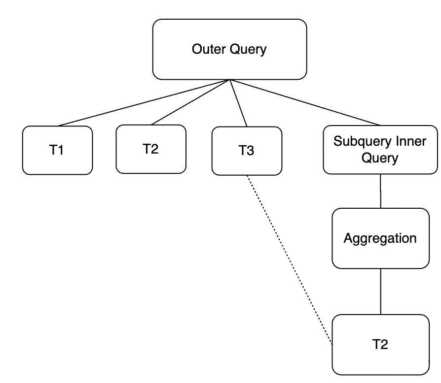
Under certain conditions, we can convert the query into the following two forms.
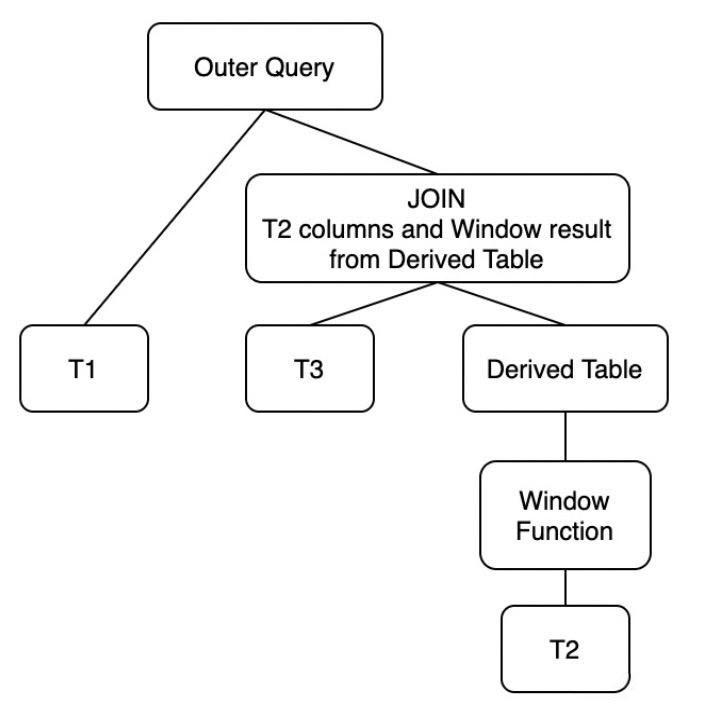
T2 Is Correlated With T3 in One or More Common Columns (Not Composing a Primary Key or Unique Key):
In this case, we can transform the original query into the first form as the following:
The Correlated Columns of T2 and T3 Compose the Primary Key or Unique Key of T3 (Forming a One-to-many Relation):
In this case, we can optimize and transform the original query to the second form:
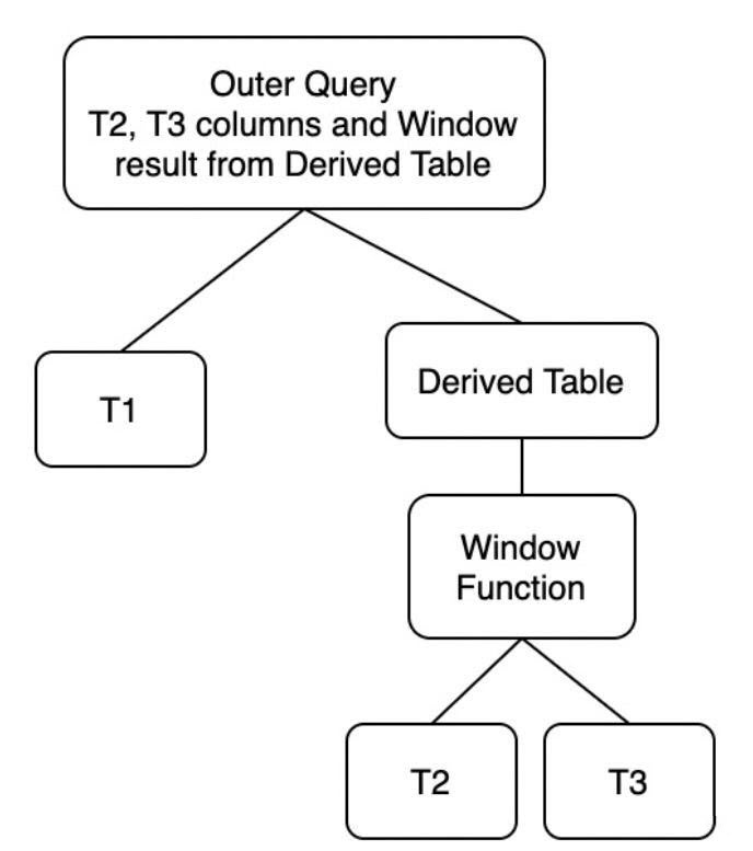
Example:
Explain format=tree SELECT s_acctbal, s_name, n_name, p_partkey, p_mfgr,
  s_address, s_phone, s_comment
FROM part, (
    SELECT MIN(ps_supplycost) OVER(PARTITION BY ps_partkey) as win_min,
      ps_partkey, ps_supplycost, s_acctbal, n_name, s_name, s_address,
      s_phone, s_comment
    FROM partsupp, supplier, nation, region
    WHERE s_suppkey = ps_suppkey
      AND s_nationkey = n_nationkey
      AND n_regionkey = r_regionkey
      AND r_name = 'ASIA') as derived
WHERE p_partkey = ps_partkey
  AND p_size = 30
  AND p_type LIKE '%STEEL'
  AND ps_supplycost = derived.win_min
ORDER BY s_acctbal DESC, n_name, s_name, p_partkey
LIMIT 100;
=============================
| -> Limit: 100 row(s)
    -> Sort: <temporary>.s_acctbal DESC, <temporary>.n_name, <temporary>.s_name, <temporary>.p_partkey, limit input to 100 row(s) per chunk
        -> Stream results
            -> Nested loop inner join
                -> Filter: (derived.win_min = derived.ps_supplycost)
                    -> Table scan on derived
                        -> Materialize
                            -> Window aggregate with buffering
                                -> Sort: <temporary>.ps_partkey
                                    -> Stream results
                                        -> Nested loop inner join  (cost=19.51 rows=35)
                                            -> Nested loop inner join  (cost=7.41 rows=16)
                                                -> Nested loop inner join  (cost=1.88 rows=5)
                                                    -> Filter: (region.r_name = 'ASIA')  (cost=0.75 rows=1)
                                                        -> Table scan on region  (cost=0.75 rows=5)
                                                    -> Index lookup on nation using i_n_regionkey (n_regionkey=region.r_regionkey)  (cost=1.12 rows=5)
                                                -> Index lookup on supplier using i_s_nationkey (s_nationkey=nation.n_nationkey)  (cost=0.85 rows=3)
                                            -> Index lookup on partsupp using i_ps_suppkey (ps_suppkey=supplier.s_suppkey)  (cost=0.56 rows=2)
                -> Filter: ((part.p_size = 30) and (part.p_type like '%STEEL'))  (cost=0.25 rows=0)
-> Single-row index lookup on part using PRIMARY (p_partkey=derived.ps_partkey) (cost=0.25 rows=1)In this way, correlated scalar subqueries can be transformed into derived tables with Group By, and multiple executions of correlated subqueries are avoided. The decorrelated derived table aggregates the correlated columns and materializes the results. The related columns and scalar computing results are retrieved for external join.
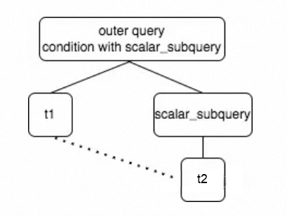
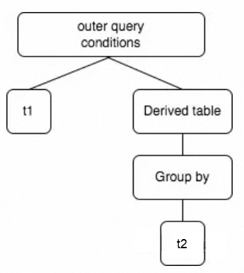
Example:
EXPLAIN format=tree
SELECT *
FROM t1
WHERE t1.c1 >
    (SELECT avg(c1)
     FROM t2
     WHERE t2.c2 = t1.c2);

=>
-> Filter: (t1.c1 > derived_1_2.Name_exp_1)
    -> Inner hash join (t1.c2 = derived_1_2.Name_exp_2)
        -> Table scan on t1  (cost=0.01 rows=19462)
        -> Hash
            -> Table scan on derived_1_2
                -> Materialize
                    -> Table scan on <temporary>
                        -> Aggregate using temporary table
-> Table scan on t2 (cost=1024.15 rows=9999)More types of ranges and lists are supported in subpartitions in combined partitions, meeting different scenarios such as time (Range)+ ID (Hash).
| Complex partition type (partition + subpartition) | PolarDB | MySQL |
| Range + Hash | Y | Y |
| List + Hash | Y | Y |
| Hash + Range | Y | N |
| Hash + List | Y | N |
| Range + Range | Y | N |
| Range + List | Y | N |
| List + Range | Y | N |
| List + List | Y | N |
| Hash + Hash | Y | N |
The parallel capabilities of DML statements and the DDL statements for adding and deleting partitions are enhanced to roll-in and roll-out partitioned tables.
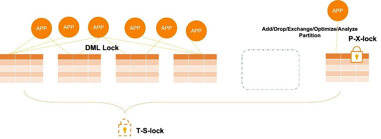
Database Administrator is required to manually and regularly add new partitions to range partitions in MySQL. Otherwise, events are used to manage the partitions. With interval partition, you no longer need the Database Administrator to intervene in the addition of new partitions. PolarDB automatically performs this operation when you insert new data, reducing the workload of the Database Administrator. The interval partition is an extension of the range partition.

Example:
CREATE TABLE t1 (order_date DATE, ...) PARTITON BY RANGE (order_date)
INTERVAL 1 MONTH (PARTITION p_first VALUES LESS THAN ( '2021-01-01');The OSS engine allows PolarDB to directly query CSV data stored in OSS, effectively reducing storage costs.
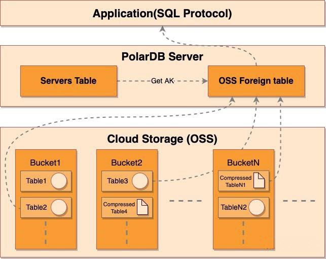
OSS foreign tables help you to perform the following operations:
• Query and analyze cold data in CSV format.
• Query and analyze compressed CSV data.
Example:
mysql> CREATE SERVER server_1                                    ### OSS server name
       FOREIGN DATA WRAPPER oss                            ### OSS server protocol name
       OPTIONS (
       DATABASE 'study',
       EXTRA_SERVER_INFO '{"oss_endpoint":"<my_oss_endpoint>",                     ### OSS configuration information
                                                "oss_bucket":"<my_oss_bucket>",
                           "oss_access_key_id":"<my_oss_acess_key_id>",
                           "oss_access_key_secret":"<my_oss_acess_key_secret>"}');

mysql> create table t1 (id int not null) engine=csv connection="server_1"

##### Then you need to manually upload the corresponding data to the OSS engine.

mysql> SELECT * FROM `t1` WHERE `id` > 5 AND `id` < 20;
+----+
| id |
+----+
| 12 |
|  6 |
|  8 |
| 10 |
+----+
4 rows in set (0.00 sec)Disadvantages of the community version
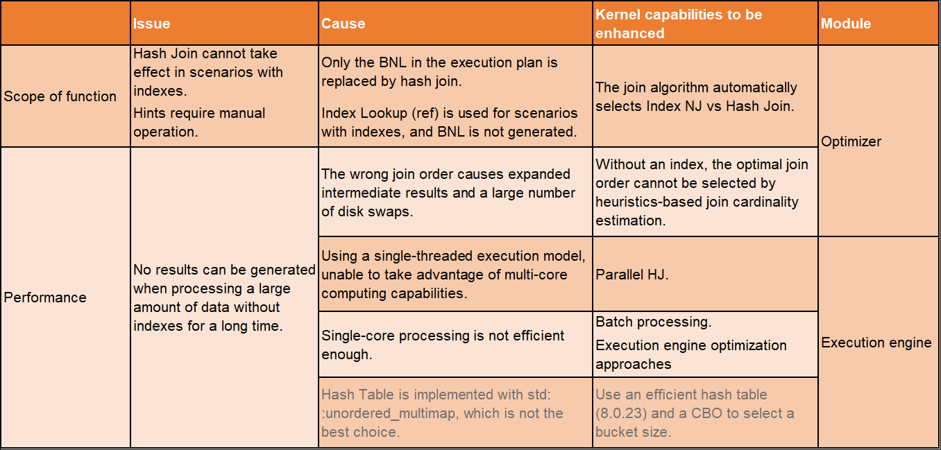
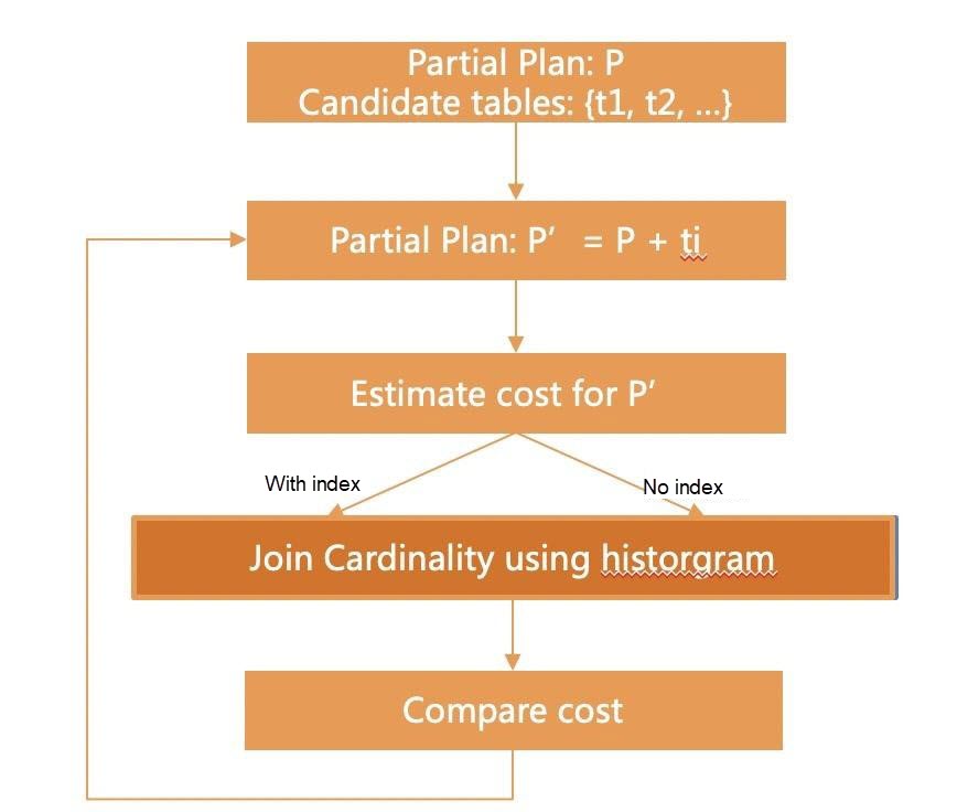
At present, to solve the inaccurate estimation of Join Cardinality (JC) and the expansion of intermediate results caused by wrong join order, you can use histograms to calculate the Join Cardinality to reduce the error rate of the join order search algorithm. It supports multi-table join and equivalent/non-equivalent conditions. Hash join is a case of this optimization.
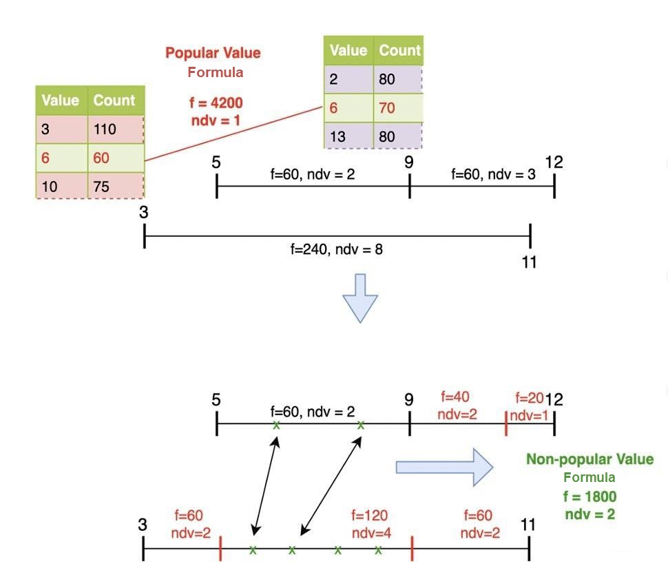
Target optimization list:
Higher accuracy of NLJ cost estimation
Cost model for two hash join scenarios
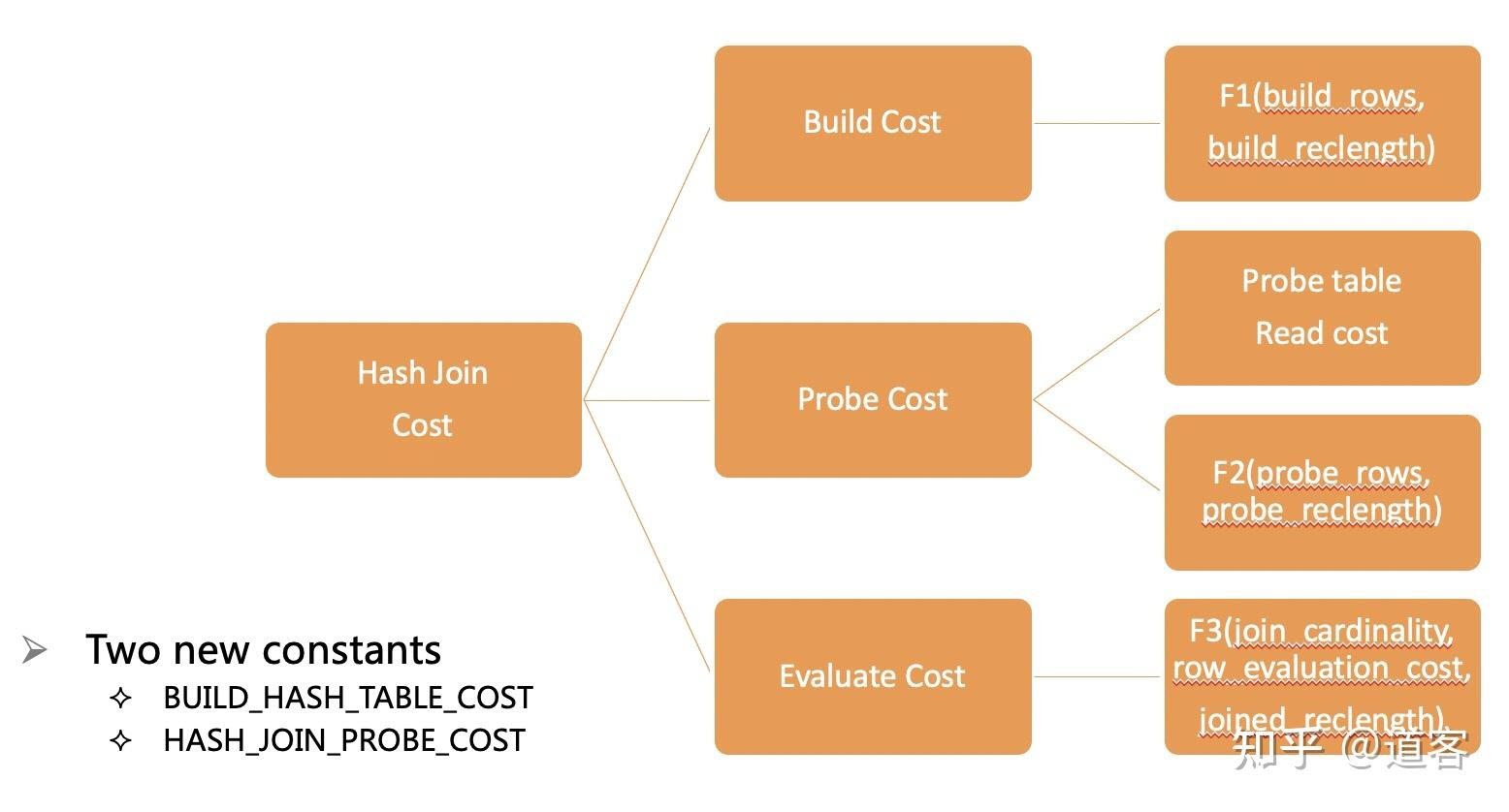
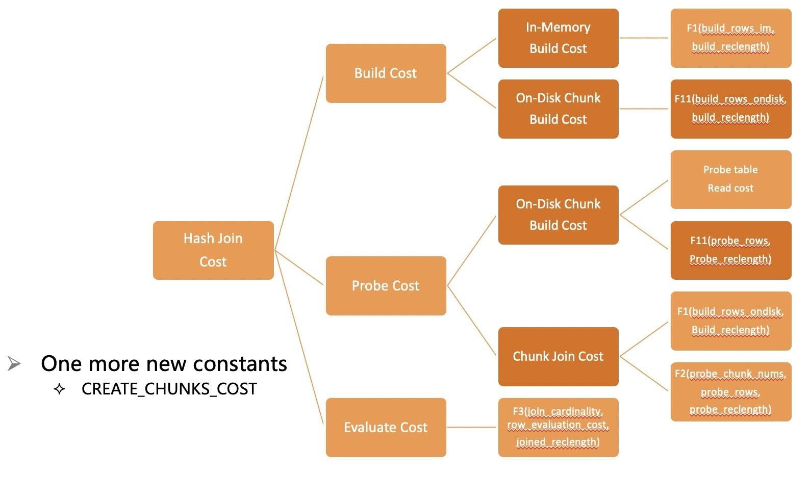
Consideration of the hash join cost in the join order search algorithm
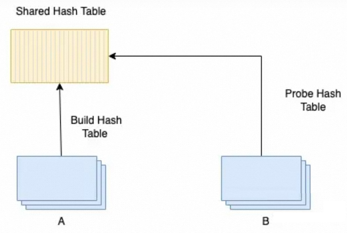
Shared hash tables, concurrent insertion by multiple build workers, and concurrent lookups by multiple probe workers are supported.
In the rule-based PHJ Plan: Post-optimization phase, marking of build tables for hash joins in the execution plan is supported.
A derived table is a subquery in the FROM clause:
SELECT ... FROM t1, (subquery) AS derived, t2 ...Two execution methods:
You can directly reference other tables in the same FROM object that precedes the lateral clause.
                  ___________________________________
                 |                OK                 |
                 v                                   |
SELECT ... FROM t1, (SELECT ... FROM ... WHERE ... = t1.col) AS derived, t2 ...
|____________NO___________|Table functions are implicitly derived tables and do not support explicitly specifying LATERAL. Currently, MySQL only supports one table function: JSON_TABLE.
SELECT people.*
FROM t1,
     JSON_TABLE(t1.json_col, '$.people[*]' COLUMNS(
                name VARCHAR(40) PATH '$.name',
                address VARCHAR(100) PATH '$.address'))
     AS people;
Lateral derived tables have the following limits:
• Lateral derived tables can only appear in the FROM clause, including tables separated by commas() or standard join statements (JOIN, INNER JOIN, CROSS JOIN, LEFT [OUTER] JOIN, and RIGHT [OUTER] JOIN).
• If the lateral derived table is located on the right side of the join operation and references the table on the left side, the join type must be INNER JOIN, CROSS JOIN, or LEFT [OUTER] JOIN.
• If the lateral derived table is on the left side of the join operation and references the table on the right side, the join type must be INNER JOIN, CROSS JOIN, or RIGHT [OUTER] JOIN.
• If a lateral derived table references an aggregate function, the aggregate query statement of the function cannot be the query statement to which the FROM clause of the lateral derived table belongs.
• According to the SQL standard, table functions have an implicit LATERAL, and the LATERAL keyword cannot exist before the function JSON_TABLE().
Example:
CREATE TABLE cites (
  city_name VARCHAR(40),
  population BIGINT,
  countr_name VARCHAR(40)
);
INSERT INTO cites VALUES
  ('Shanghai', 24183300, 'China'),
  ('Beijing', 20794000, 'China'),
  ...
;

The largest City of Each Country
Option #1:
SELECT dt.population, dt.city_name, c.country_name
FROM
  (SELECT DISTINCT country_name FROM cities) AS c,
  LATERAL (
    SELECT city_name, population
    FROM cities
    WHERE cities.country_name = c.country_name
    ORDER BY population DESC
    LIMIT 1
  ) AS dt;

Option #2:
SELECT dt.pop, dt2.city_name, dt.country_name
FROM
  (
    SELECT country_name, MAX(population) AS pop
    FROM cities
    GROUP BY country_name
  ) AS dt,
  LATERAL (
    SELECT city_name
    FROM cities
    WHERE cities.country_name = dt.country_name
      AND cities.population = dt.pop
  ) AS dt2;

Option #3:
SELECT dt.pop, dt2.city_name, dt.country_name
FROM
  (
    SELECT country_name, MAX(population) AS pop
    FROM cities
    GROUP BY country_name
  ) AS dt
  JOIN cities
    ON cities.country_name = dt.country_name
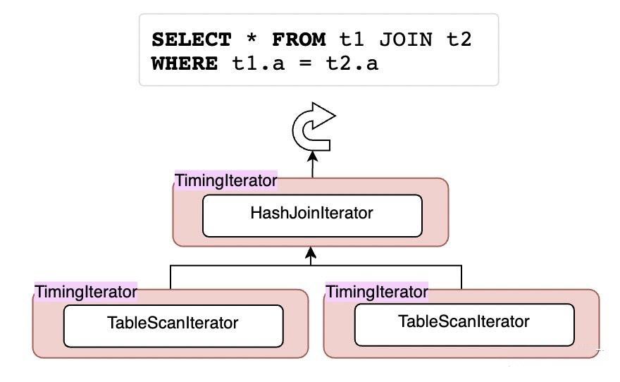
AND cities.population = dt.pop;After version 8.0.18, the MySQL executor is basically composed of iterators, and each operation is an iterator. Each read starts from the root node line by line. The main interfaces are Init() and Read().
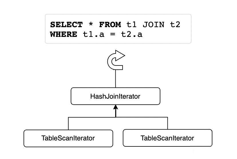
Iterators are organized in a tree form. Generally, iterators have only one child (JOIN iterators have two children, which are the outer and inner tables of JOIN respectively). All iterators directly accessed during recursive traversal are subclasses of RowIterator.
The following is an example of Explain Format Tree:
SELECT l_orderkey,
       sum(l_extendedprice * (1 - l_discount)) AS revenue,
       o_orderdate,
       o_shippriority
FROM customer,
     orders,
     lineitem
WHERE c_mktsegment = 'AUTOMOBILE'
  AND c_custkey = o_custkey
  AND l_orderkey = o_orderkey
  AND o_orderdate < '1995-03-09'
  AND l_shipdate > '1995-03-09'
GROUP BY l_orderkey,
         o_orderdate,
         o_shippriority
ORDER BY revenue DESC,
         o_orderdate
LIMIT 10
=============================================================
-> Limit: 10 row(s)  (cost=4100325.74 rows=10)
    -> Gather (merge sort; slice: 1; workers: 8; actual workers: 32)  (cost=4100325.74 rows=80)
        -> Limit: 10 row(s)  (cost=4100302.92 rows=10)
            -> Sort: <temporary>.revenue DESC, <temporary>.o_orderdate, limit input to 10 row(s) per chunk  (cost=4100302.92 rows=276201)
                -> Table scan on <temporary>
                    -> Aggregate using temporary table  (cost=3927278.15 rows=276201)
                        -> Repartition (hash keys: lineitem.l_orderkey, orders.o_orderDATE, orders.o_shippriority; slice: 2; workers: 8)  (cost=3899658.05 rows=276201)
                            -> Table scan on <temporary>
                                -> Aggregate using temporary table  (cost=3844407.77 rows=276201)
                                    -> Nested loop inner join  (cost=2049078.68 rows=2762014)
                                        -> Nested loop inner join  (cost=1150571.52 rows=1372006)
                                            -> Filter: (customer.c_mktsegment = 'AUTOMOBILE')  (cost=18991.65 rows=184397)
                                                -> Parallel table scan on customer, with parallel partitions: 158  (cost=18991.65 rows=1843968)
                                            -> Filter: (orders.o_orderDATE < DATE'1995-03-09')  (cost=3.75 rows=8)
                                                -> Index lookup on orders using i_o_custkey (o_custkey=customer.c_custkey)  (cost=3.75 rows=15)
                                        -> Filter: (lineitem.l_shipDATE > DATE'1995-03-09')  (cost=0.25 rows=2)
                                            -> Index lookup on lineitem using PRIMARY (l_orderkey=orders.o_orderkey)  (cost=0.25 rows=4)
EXPLAIN ANALYZE is a new tool provided in MySQL 8.0.18 and later versions. It is an analysis tool for query performance that can show in detail where and how much time is spent during the execution of query statements. EXPLAIN ANALYZE makes a query plan and executes it to measure the actual metrics of each key point in the query plan, such as time consumption and the number of returned instances, and finally prints out the details, including:
• The actual time of obtaining the first row (unit: millisecond)
• The actual time of obtaining all the rows (unit: millisecond)
• The number of rows actually read
• The actual number of cycles
It wraps a TimingIterator for statistical purposes:
test:tpch_1> explain analyze select         s_acctbal,         s_name,         n_name,         p_partkey,         p_mfgr,         s_address,         s_phone,         s_comment from         part,         supplier,         partsupp,         nation,         region where         p_partkey = ps_partkey         and s_suppkey = ps_suppkey         and p_size = 15         and p_type like '%BRASS'         and s_nationkey = n_nationkey         and n_regionkey = r_regionkey         and r_name = 'EUROPE'         and ps_supplycost = (                 select                         min(ps_supplycost)                 from                         partsupp,                         supplier,                         nation,                         region                 where                         p_partkey = ps_partkey                         and s_suppkey = ps_suppkey                         and s_nationkey = n_nationkey                         and n_regionkey = r_regionkey                         and r_name = 'EUROPE'         ) order by         s_acctbal desc,         n_name,         s_name,         p_partkey limit 100\G
*************************** 1. row ***************************
EXPLAIN: -> Limit: 100 row(s)  (actual time=2042.733..2042.818 rows=100 loops=1)
    -> Sort: derived_1_2.Name_exp_3 DESC, derived_1_2.Name_exp_5, derived_1_2.Name_exp_4, derived_1_2.Name_exp_6, limit input to 100 row(s) per chunk  (actual time=0.785..0.820 rows=100 loops=1)
        -> Filter: (derived_1_2.Name_exp_1 = derived_1_2.Name_exp_2)  (actual time=0.004..0.392 rows=460 loops=1)
            -> Table scan on derived_1_2  (actual time=0.002..0.196 rows=642 loops=1)
                -> Materialize  (actual time=2042.731..2042.787 rows=100 loops=1)
                    -> Window aggregate with buffering  (actual time=2036.026..2041.136 rows=642 loops=1)
                        -> Sort: <temporary>.ps_partkey  (actual time=2035.974..2036.243 rows=642 loops=1)
                            -> Stream results  (actual time=5.913..2034.496 rows=642 loops=1)
                                -> Nested loop inner join  (cost=31.61 rows=2) (actual time=5.903..2031.468 rows=642 loops=1)
                                    -> Nested loop inner join  (cost=19.51 rows=35) (actual time=0.177..1182.434 rows=158960 loops=1)
                                        -> Nested loop inner join  (cost=7.41 rows=16) (actual time=0.114..12.712 rows=1987 loops=1)
                                            -> Nested loop inner join  (cost=1.88 rows=5) (actual time=0.083..0.113 rows=5 loops=1)
                                                -> Filter: (region.r_name = 'EUROPE')  (cost=0.75 rows=1) (actual time=0.051..0.061 rows=1 loops=1)
                                                    -> Table scan on region  (cost=0.75 rows=5) (actual time=0.043..0.051 rows=5 loops=1)
                                                -> Index lookup on nation using i_n_regionkey (n_regionkey=region.r_regionkey)  (cost=1.12 rows=5) (actual time=0.030..0.046 rows=5 loops=1)
                                            -> Index lookup on supplier using i_s_nationkey (s_nationkey=nation.n_nationkey)  (cost=0.85 rows=3) (actual time=0.021..2.396 rows=397 loops=5)
                                        -> Index lookup on partsupp using i_ps_suppkey (ps_suppkey=supplier.s_suppkey)  (cost=0.56 rows=2) (actual time=0.014..0.566 rows=80 loops=1987)
                                    -> Filter: ((part.p_size = 15) and (part.p_type like '%BRASS'))  (cost=0.25 rows=0) (actual time=0.005..0.005 rows=0 loops=158960)
                                        -> Single-row index lookup on part using PRIMARY (p_partkey=partsupp.ps_partkey)  (cost=0.25 rows=1) (actual time=0.004..0.004 rows=1 loops=158960)

1 row in set, 1 warning (2.08 sec)
Analysis Toolbox:

JSON array indexes are based on a multi-valued index mechanism. See the following example:
{
    "user":"Bob",
    "user_id":31,
    "zipcode":[94477,94536]
}
Example of using this index:
mysql> CREATE TABLE customers (
    ->     id BIGINT NOT NULL AUTO_INCREMENT PRIMARY KEY,
    ->     modified DATETIME DEFAULT CURRENT_TIMESTAMP ON UPDATE CURRENT_TIMESTAMP,
    ->     custinfo JSON
    ->     );
Query OK, 0 rows affected (0.51 sec)

mysql> INSERT INTO customers VALUES
    ->     (NULL, NOW(), '{"user":"Jack","user_id":37,"zipcode":[94582,94536]}'),
    ->     (NULL, NOW(), '{"user":"Jill","user_id":22,"zipcode":[94568,94507,94582]}'),
    ->     (NULL, NOW(), '{"user":"Bob","user_id":31,"zipcode":[94477,94507]}'),
    ->     (NULL, NOW(), '{"user":"Mary","user_id":72,"zipcode":[94536]}'),
    ->     (NULL, NOW(), '{"user":"Ted","user_id":56,"zipcode":[94507,94582]}');
Query OK, 5 rows affected (0.07 sec)
Records: 5  Duplicates: 0  Warnings: 0
You can use JSON_CONTAINS(...)/JSON_OVERLAPS(...)/MEMBER OF(...) to search. The following shows the usage of the corresponding index of zips in the explain statements:
test:tpch_1> explain  SELECT * FROM customers WHERE 94507 MEMBER OF(custinfo->'$.zipcode');
+----+-------------+-----------+------------+------+---------------+------+---------+-------+------+----------+-------------+
| id | select_type | table     | partitions | type | possible_keys | key  | key_len | ref   | rows | filtered | Extra       |
+----+-------------+-----------+------------+------+---------------+------+---------+-------+------+----------+-------------+
|  1 | SIMPLE      | customers | NULL       | ref  | zips          | zips | 9       | const |    1 |   100.00 | Using where |
+----+-------------+-----------+------------+------+---------------+------+---------+-------+------+----------+-------------+
1 row in set, 1 warning (0.03 sec)

test:tpch_1> explain SELECT * FROM customers WHERE JSON_CONTAINS(custinfo->'$.zipcode', CAST('[94507,94582]' AS JSON));
+----+-------------+-----------+------------+-------+---------------+------+---------+------+------+----------+-------------+
| id | select_type | table     | partitions | type  | possible_keys | key  | key_len | ref  | rows | filtered | Extra       |
+----+-------------+-----------+------------+-------+---------------+------+---------+------+------+----------+-------------+
|  1 | SIMPLE      | customers | NULL       | range | zips          | zips | 9       | NULL |    6 |   100.00 | Using where |
+----+-------------+-----------+------------+-------+---------------+------+---------+------+------+----------+-------------+
1 row in set, 1 warning (0.03 sec)

test:tpch_1> explain SELECT * FROM customers WHERE JSON_OVERLAPS(custinfo->'$.zipcode', CAST('[94507,94582]' AS JSON));
+----+-------------+-----------+------------+-------+---------------+------+---------+------+------+----------+-------------+
| id | select_type | table     | partitions | type  | possible_keys | key  | key_len | ref  | rows | filtered | Extra       |
+----+-------------+-----------+------------+-------+---------------+------+---------+------+------+----------+-------------+
|  1 | SIMPLE      | customers | NULL       | range | zips          | zips | 9       | NULL |    6 |   100.00 | Using where |
+----+-------------+-----------+------------+-------+---------------+------+---------+------+------+----------+-------------+
1 row in set, 1 warning (0.03 sec)

Example of not using the index:
test:tpch_1> explain  SELECT * FROM customers_noindex WHERE 94507 MEMBER OF(custinfo->'$.zipcode');
+----+-------------+------------+------------+------+---------------+------+---------+------+------+----------+-------------+
| id | select_type | table      | partitions | type | possible_keys | key  | key_len | ref  | rows | filtered | Extra       |
+----+-------------+------------+------------+------+---------------+------+---------+------+------+----------+-------------+
|  1 | SIMPLE      | customers1 | NULL       | ALL  | NULL          | NULL | NULL    | NULL |    1 |   100.00 | Using where |
+----+-------------+------------+------------+------+---------------+------+---------+------+------+----------+-------------+
1 row in set, 1 warning (0.03 sec)Before version 8.0.18, MySQL only supported the Nest Loop Join algorithm. Many optimizations were made for this algorithm, such as Block Nest Loop Join, Index Nest Loop Join, and Batched Key Access. However, Hash Join is officially supported in version 8.0.18 and later versions.
The following describes how Hash Join works:
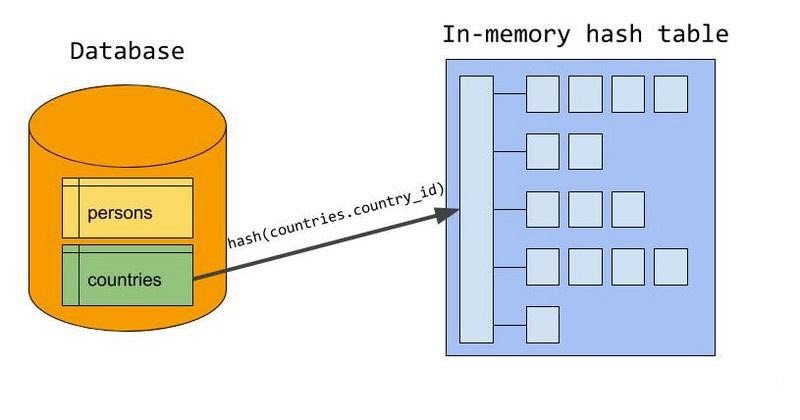
Generally, hash joins are divided into two phases: the build phase and the probe phase. In the build phase, the JOIN condition attribute value is used as the key value of the hash table to construct a full-memory hash table. Each row retains the input of one of the tables. Generally, the smaller one of the two tables is used for the input (in bytes, not rows).
Example:
ELECT
  given_name, country_name
FROM
  persons JOIN countries ON persons.country_id = countries.country_id;
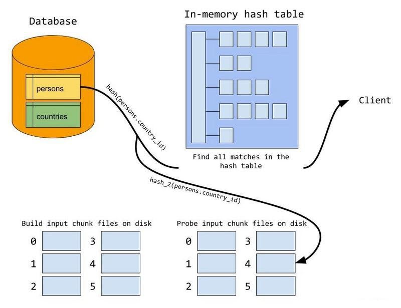
Select countries as the build table to build the hash table, and country_id as the join condition, which becomes the hash key. After all rows are stored in the hash table, the build phase is over.
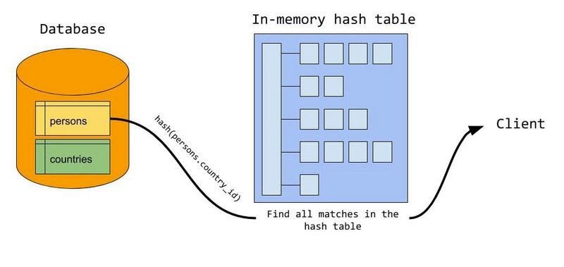
In the probe phase, rows are read from the probe table, and each row is checked for matching keys in the hash table. If a matching row is found, the values are merged and returned to the client.
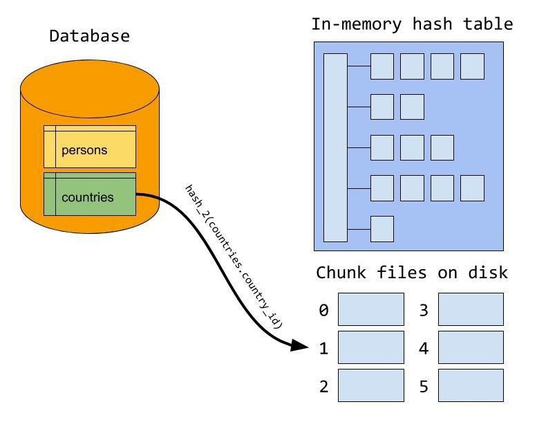
The above algorithm assumes that the entire hash table can be saved to memory. You can use join_buffer_size for control, but if the memory storage is full, the rest will be stored on the disk.
Back to the build phase, the input to the build table is hashed into chunks and written to multiple chunk files on disk. Then, attempts are made to set the serial number of every chunk so that the largest chunk fits exactly the memory. The maximum of chunk files is strictly limited to 128. By using a different hash function than the one used during the memory build phase, the hash value of the join attribute is computed to determine which chunk file the row is written to.
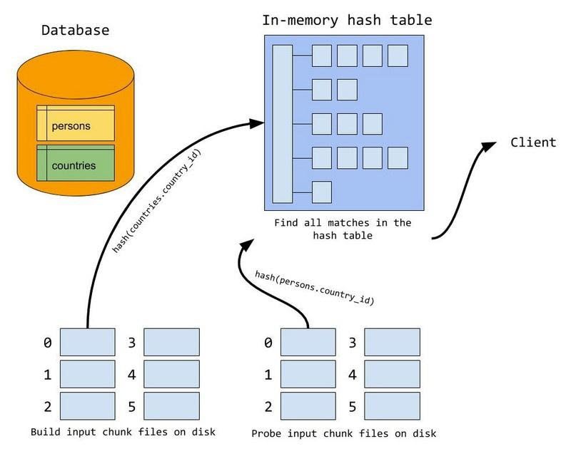
In the probe phase, the rows that the probe meets may be written in the build table chunk file of the disk. Therefore, each probe input needs to use the same hash function to be partitioned and written to the disk. That means we can perform a memory hash join matching on a pair of build/probe chunk files.
To this end, after the probe phase ends, we start reading from the disk and using the matching algorithm of memory hash join to match pairs of build/probe chunk files on the disk in turn.
Example:
mysql> EXPLAIN FORMAT=TREE
    -> SELECT *
    ->     FROM t1
    ->     JOIN t2
    ->         ON (t1.c1 = t2.c1 AND t1.c2 < t2.c2)
    ->     JOIN t3
    ->         ON (t2.c1 = t3.c1)\G
*************************** 1. row ***************************
EXPLAIN: -> Inner hash join (t3.c1 = t1.c1)  (cost=1.05 rows=1)
    -> Table scan on t3  (cost=0.35 rows=1)
    -> Hash
        -> Filter: (t1.c2 < t2.c2)  (cost=0.70 rows=1)
            -> Inner hash join (t2.c1 = t1.c1)  (cost=0.70 rows=1)
                -> Table scan on t2  (cost=0.35 rows=1)
                -> Hash
                    -> Table scan on t1  (cost=0.35 rows=1)
In addition, PolarDB for MySQL 8.0.2 also backports the subsequent official support for hash joins due to the limits of version 8.0.18. At least one equi-join condition is no longer required to use hash joins.
• Inner non-equi-join:
mysql> EXPLAIN FORMAT=TREE SELECT * FROM t1 JOIN t2 ON t1.c1 < t2.c1\G
*************************** 1. row ***************************
EXPLAIN: -> Filter: (t1.c1 < t2.c1)  (cost=4.70 rows=12)
    -> Inner hash join (no condition)  (cost=4.70 rows=12)
        -> Table scan on t2  (cost=0.08 rows=6)
        -> Hash
            -> Table scan on t1  (cost=0.85 rows=6)
• Semi-join:
mysql> EXPLAIN FORMAT=TREE SELECT * FROM t1
    ->     WHERE t1.c1 IN (SELECT t2.c2 FROM t2)\G
*************************** 1. row ***************************
EXPLAIN: -> Nested loop inner join
    -> Filter: (t1.c1 is not null)  (cost=0.85 rows=6)
        -> Table scan on t1  (cost=0.85 rows=6)
    -> Single-row index lookup on <subquery2> using <auto_distinct_key> (c2=t1.c1)
        -> Materialize with deduplication
            -> Filter: (t2.c2 is not null)  (cost=0.85 rows=6)
                -> Table scan on t2  (cost=0.85 rows=6)
• Anti-join:
mysql> EXPLAIN FORMAT=TREE SELECT * FROM t2
    ->     WHERE NOT EXISTS (SELECT * FROM t1 WHERE t1.col1 = t2.col1)\G
*************************** 1. row ***************************
EXPLAIN: -> Nested loop antijoin
    -> Table scan on t2  (cost=0.85 rows=6)
    -> Single-row index lookup on <subquery2> using <auto_distinct_key> (c1=t2.c1)
        -> Materialize with deduplication
            -> Filter: (t1.c1 is not null)  (cost=0.85 rows=6)
                -> Table scan on t1  (cost=0.85 rows=6)
• Left outer join
mysql> EXPLAIN FORMAT=TREE SELECT * FROM t1 LEFT JOIN t2 ON t1.c1 = t2.c1\G
*************************** 1. row ***************************
EXPLAIN: -> Left hash join (t2.c1 = t1.c1)  (cost=3.99 rows=36)
    -> Table scan on t1  (cost=0.85 rows=6)
    -> Hash
        -> Table scan on t2  (cost=0.14 rows=6)
• Right outer join (note that MySQL rewrites all right outer joins as left outer joins):
mysql> EXPLAIN FORMAT=TREE SELECT * FROM t1 RIGHT JOIN t2 ON t1.c1 = t2.c1\G
*************************** 1. row ***************************
EXPLAIN: -> Left hash join (t1.c1 = t2.c1)  (cost=3.99 rows=36)
    -> Table scan on t2  (cost=0.85 rows=6)
    -> Hash
-> Table scan on t1 (cost=0.14 rows=6)About Database Kernel | PolarDB HTAP Serverless: Build a Cost-efficient Real-Time Analysis System
About Database Kernel | Transaction System of PolarDB-X Storage Engine - Part1
ApsaraDB - February 4, 2024
ApsaraDB - January 22, 2021
JDP - February 10, 2022
JDP - December 23, 2021
JDP - July 9, 2021
Morningking - September 26, 2023
 PolarDB for PostgreSQL
Alibaba Cloud PolarDB for PostgreSQL is an in-house relational database service 100% compatible with PostgreSQL and highly compatible with the Oracle syntax.
Learn More PolarDB for Xscale
Alibaba Cloud PolarDB for Xscale (PolarDB-X) is a cloud-native high-performance distributed database service independently developed by Alibaba Cloud.
Learn More PolarDB for MySQL
Alibaba Cloud PolarDB for MySQL is a cloud-native relational database service 100% compatible with MySQL.
Learn More Database for FinTech Solution
Leverage cloud-native database solutions dedicated for FinTech.
Learn MoreMore Posts by ApsaraDB