By Ahmed F. Gad, Alibaba Cloud Community Blog author
Welcome again in a new part of the series in which the Fruits360 dataset will be classified in Keras running in Jupyter notebook using features extracted by transfer learning of MobileNet which is a pre-trained convolutional neural network (CNN).
Part 1 discussed the traditional machine learning (ML) pipeline and highlighted that manual feature extraction is not the right choice for working with large datasets. On the other hand, deep learning (DL) able to automatically extract features from such large datasets. Part 1 also introduced transfer learning to highlight its benefits for making it possible to use DL for small datasets by transferring the learning of a pre-trained model.
In this tutorial, which is Part 2 of the series, we will start the first practical side of the project. This is by starting working with creating a Jupyter notebook and making sure everything is up and running. After that, the Fruits360 dataset is downloaded using Keras within the Jupyter notebook. After making sure the dataset is downloaded successfully, its training and test images are read into NumPy arrays which will be fed later to MobileNet for extracting features.
The sections covered in this tutorial are as follows:
This series uses the Jyputer notebook for transfer learning of the pre-trained MobileNet. It is recommended to use the Jupyer notebook environment on Alibaba Cloud in order to start working in this series. Preparing the notebook environment starts by creating an instance of the Elastic Compute Service (ECS) provided by Alibaba Cloud. What is an ECS? ECS is magic that offers the users with whatever they need to do high-speed computing on the cloud and also more dynamic features.
The interesting news is that Alibaba Cloud allows new users to start a free trial with 300$ in their wallet. You can build your first ECS instance with CPU, memory, and disk storage according to your need.
The steps for starting your free trial is very simple. Just create an Alibaba Cloud account by registering in its official site http://alibabacloud.com. After that, you can go to your account settings to add a payment method. Don’t worry. You will not get charged for starting the free trial. There is just a transaction of 1$ that the system will create automatically after adding the payment method to make sure your account is valid. It transaction will be canceled after 24 hours.
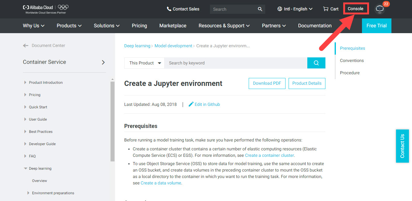
After adding the payment method, you can start your free trial from this page https://www.alibabacloud.com/campaign/free-trial. After that, you can go to your console from the button highlighted in the next figure to set up your first ECS instance.
The console is where you can control all of the services available in your account. The next figure shows how the page appears.
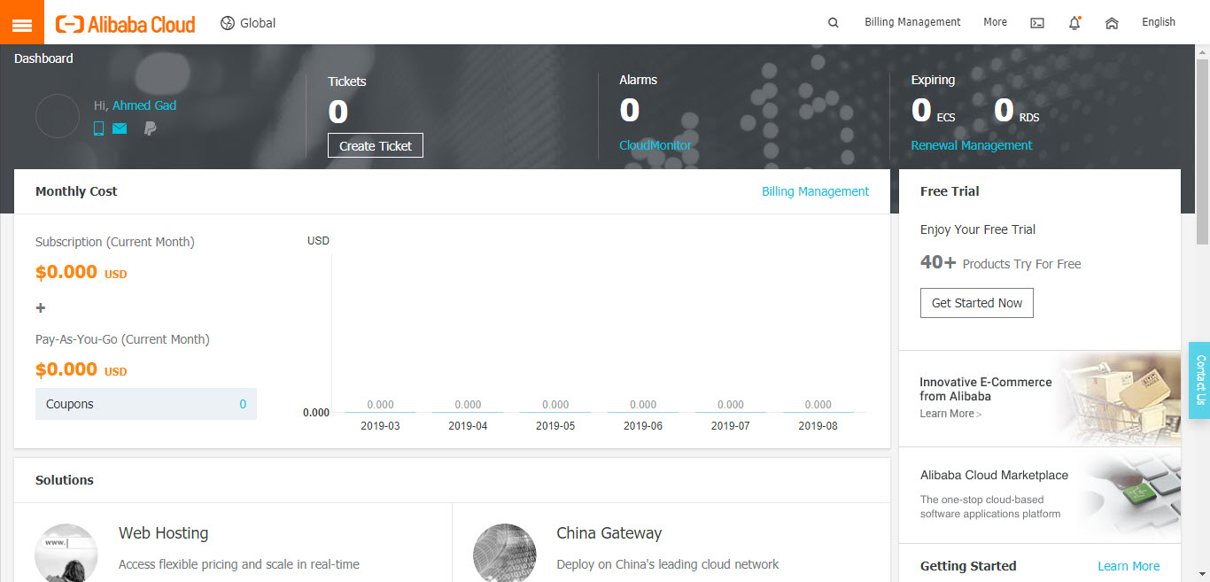
Just click on the 3 lines at the top-left corner to see the menu from which you can go to your ECS instances as shown in the next figure.
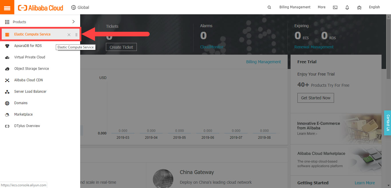
By clicking on the Elastic Computer Service button shown above, you will be directed to the page from which you can control and manage your ECS instances as shown in the next figure.
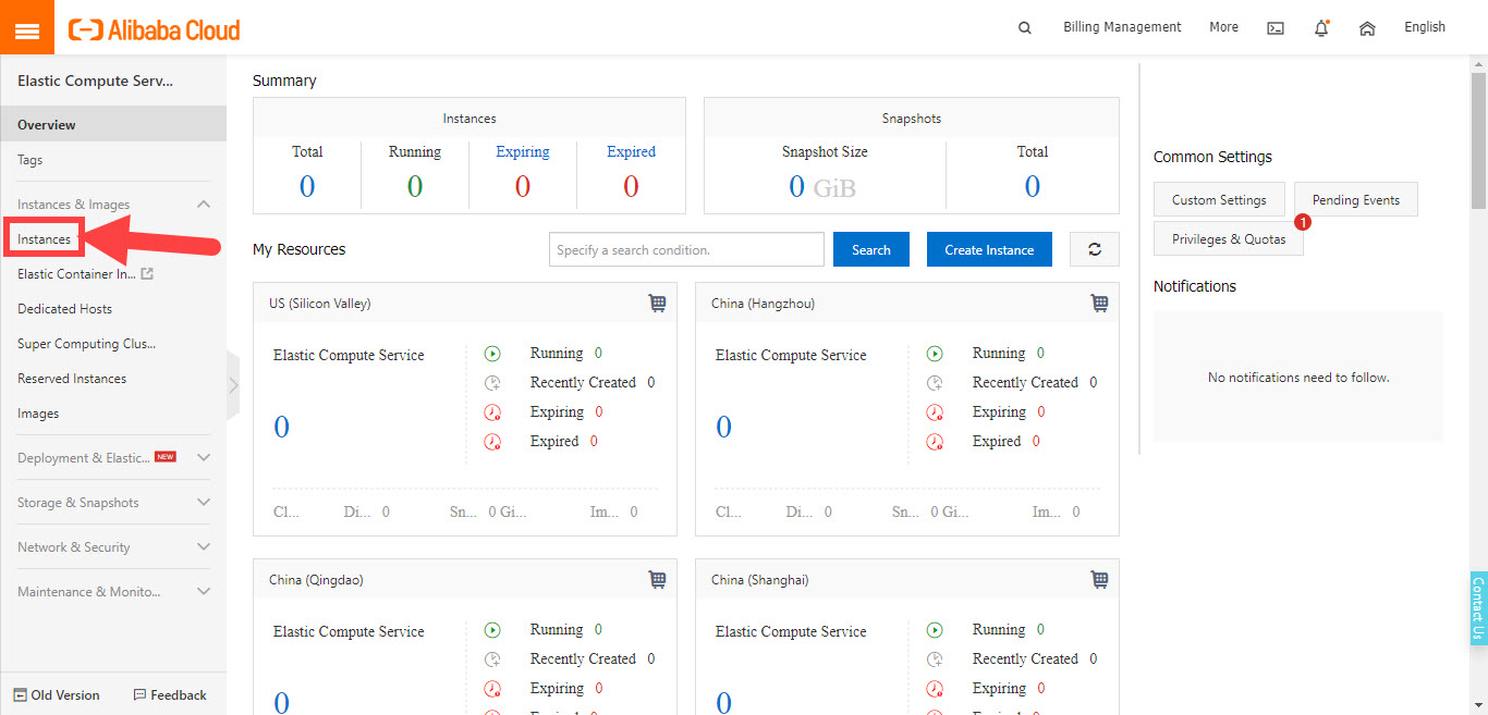
In order to create your first ECS instance, just click on the Instances option which appears at the top of the left menu. The page will be as shown below.
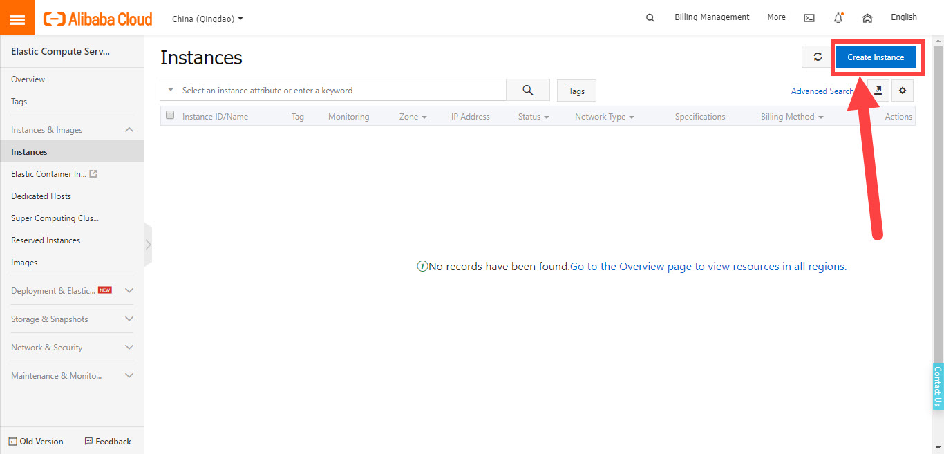
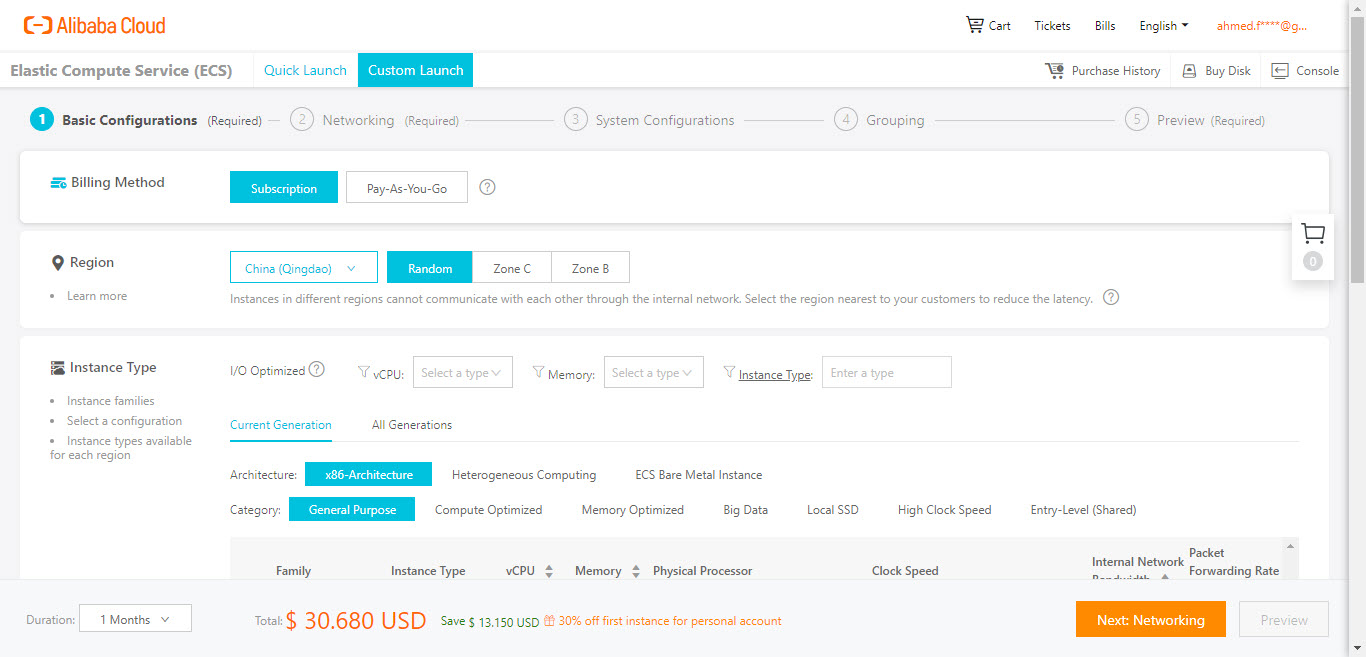
Click on the Create Instance button to get redirected to the page from which you can build your first ECS instance. From here, you can select the amount of RAM, disk storage, the region of the cloud based on your location, and everything required to run a remote OS. In the free trial, you will pay NOTHING in order to start your ECS.
Jupyter notebooks are web-based IDE that can work with different languages such as Python, Scala, R, and more. This is using the concept of kernel. Different kernels allow the notebook to work with different languages.
Through this series, Python will be used. You can create a notebook that is prepared with most recent libraries for use including TensorFlow, Keras, NumPy, scikit-learn, and more. If a library is not currently existing, it can be simply installed.
In such notebooks, you can write interactive code not only written in Python because Jupyter supports a number of kernels for different languages. In addition to writing code, you can also write text, add images, or links. So, it is not only about code writing but about building interactive documents.
In order to start working with Jupyter notebooks in Alibaba Cloud, you can follow the instructions found in these links. They provide detailed steps for creating the Jupyter notebooks and installing the required libraries. Through this series, we are going to use Python 3.
The extension of the notebook is ipynb which stands for Interactive Python NoteBook. Note that Jyputer notebooks are an extension to the IPython (Interactive Python) project and this is why their names are combined in the extension of the Jupyter notebooks. A Jupyter notebook consists of cells. Within each cell, you can either write code or text.
This project targets classifying images. This section will do a basic step which is just read and processing an image. Because there is no image available at the notebook, then you can upload an image to the notebook easily.
The code listed below is the code cell content that reads the image using Keras and displays it using Matplotlib. The image is read using the Keras load_img() function. This function returns the image as PIL object. To convert it into a NumPy array, the img_to_array() function is used.
After being converted into a NumPy array, the image shape and data type are printed. Note that the data type of the returned image is float32 despite having their pixel values ranging from 0.0 to 255.0. To force the range to be from 0.0 to 1.0, the image is divided by 255.0. The pixel at location (50, 50) is printed before and after the division.
Finally, the image is shown using the imshow() function in the Matplotlib library.
import numpy
import keras
import matplotlib.pyplot

img = keras.preprocessing.image.load_img("0_100.jpg")
img_array = keras.preprocessing.image.img_to_array(img)

print(img_array.shape, img_array.dtype)

print(img_array[50, 50])

img_array = img_array/255.0

print(img_array[50, 50])

matplotlib.pyplot.imshow(img_array)
matplotlib.pyplot.show()
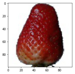
In order to run the cell, just click on the arrow button on the top left side of the cell. The result of the print messages is given below. The image shape is 100x100x3 and its dtype which is float32. The image is actually a sample from the Strawberry class of the Fruits360 dataset as shown below.
(100, 100, 3) float32
[115.   6.  12.]
[0.4509804  0.02352941 0.04705882]
After successfully reading an image, let's start downloading the dataset and then reading all of its images.
If you want to work on data in the Jupyter notebook, one way is to upload it using the upload UPLOAD as discussed previously. Unfortunately, it is not the preferred option to upload large files or datasets. At first, the data will be lost after recycling the notebook and thus you have to upload it again. It is tiresome to do especially for slow Internet connections.
If you are running the notebook in Alibaba Cloud, then we can classify the data in which we want to work on to 2 categories:
If the data to be processed is not available on the Web but in our PC, then we have to upload it for use in the notebook running in Alibaba Cloud. But if the notebook is recycled, we have to upload the data again.
If the data to be processed is available on the Web, then we can avoid uploading it to the notebook. We can download it while running the code cell. This is what we are going to do. Our mission is to search the Web to find the link from which the data can be downloaded.
If you are running the notebook locally in your PC, then the above classification does not work for you as if the data is available in your PC then you will not upload it to anywhere. But if the data is not available in your PC, then you need to download it.
Regarding the Fruits360 dataset, it is available in Kaggle in this page https://www.kaggle.com/moltean/fruits. At first, its name has the number 360 because each class of fruits has images that cover all 360 angles.
The version we are going to use is version number 48 which has 102 classes which was released on 6 May 2019. It is available in this page https://www.kaggle.com/moltean/fruits/version/48.
Of the 70,513 samples in Fruits360 version 48, there are 52,718 for training and 17,692 for testing. Each training and testing image has just one type of fruit. Note that the sum of the training and testing samples is just 70,410. The remaining images contain more than 1 type of fruits and they are excluded from our experiments.
By scrolling down in the Fruits360 version 48 page, you will find a section from which you can download the dataset as shown in the next figure. By clicking on the download button, the file will start downloading. Note that it will start downloading in your own machine. Because we do not need to download it to our machine, then cancel downloading the file. We are doing this in order to find the link from which notebook can download the dataset.
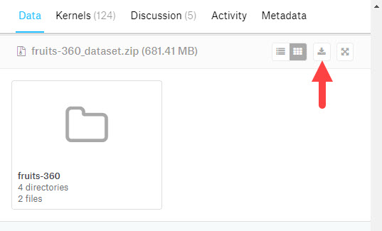
After canceling the download, copy the link of the canceled download. If you are using a web browser for downloading the file, then copying the download link is simply done as shown in the next figure. Just right-click the download link and select the "Copy link address" option from the menu. Note that the download link changes every few days and thus if you found that the link is expired, then repeat the previous steps to get the new link.
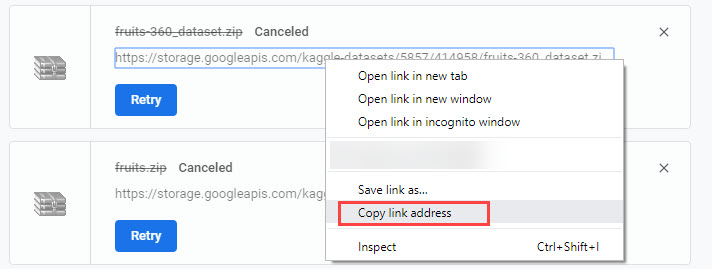
The link I got is available HERE. I think it will be expired at the time you are reading this tutorial. Simply repeat of this section again and you will get the new link. What after getting the download link? The next step is to download the dataset. This is discussed in the next section.
After getting the download link, next is to download the Fruits360 dataset. The code for downloading the dataset is listed below. The file is downloaded using the get_file(). It downloads the file if it is not currently existing in the cache. This function accepts 2 must-specify arguments in addition to 8 other optional arguments. The 2 arguments that the user must specify are as follows:
The origin is set to the link we got in the previous section. Note that you have to replace the URL in this code by the link you got to make sure it is still a valid link.
The fname could be set to any name with an extension that matches the downloaded file. From the previous figure, the dataset is downloaded as a compressed ZIP file. We can make use of the extract optional argument by setting its value to True to extract the file once it is downloaded.
import tensorflow as tf
import os

zip_file = tf.keras.utils.get_file(origin="https://storage.apis.com/kaggle-datasets/5857/414958/fruits-360_dataset.zip?AccessId=web-data@kaggle-161607.iam.gserviceaccount.com&Expires=1566314394&Signature=rqm4aS%2FIxgWrNSJ84ccMfQGpjJzZ7gZ9WmsKok6quQMyKin14vJyHBMSjqXSHR%2B6isrN2POYfwXqAgibIkeAy%2FcB2OIrxTsBtCmKUQKuzqdGMnXiLUiSKw0XgKUfvYOTC%2F0gdWMv%2B2xMLMjZQ3CYwUHNnPoDRPm9GopyyA6kZO%2B0UpwB59uwhADNiDNdVgD3GPMVleo4hPdOBVHpaWl%2F%2B%2BPDkOmQdlcH6b%2F983JHaktssmnCu8f0LVeQjzZY96d24O4H85x8wdZtmkHZCoFiIgCCMU%2BKMMBAbTL66QiUUB%2FW%2FpULPlpzN9sBBUR2yydB3CUwqLmSjAcwz3wQ%2FpIhzg%3D%3D", fname="fruits-360.zip", extract=True)
base_dir, _ = os.path.splitext(zip_file)
print(base_dir)
After placing the above code into a code cell and running it, the dataset will be downloaded and the messages below will be printed.
714514432/714509197 [==============================] - 7s 0us/step
/root/.keras/datasets/fruits-360
After the file is downloaded successfully, the splitext() function inside the os module is used to return the path of the directory in which the dataset is downloaded. The path of the dataset is /root/.keras/datasets/fruits-360. Note that inside the dataset is firstly downloaded as a ZIP file and then extracted after setting the extract argument passed to the get_file() function to True.
Note that after downloading and extracting the dataset, the free space in the notebook disk will be reduced. For me, it is reduced from 23.56 to 22.06 GB. That is 1.5 GB because the compressed file is about 700 MB and the extracted file is a bit larger than this size.
To see the contents of the datasets directory, the next code is executed. The contents of the datasets directory are returned using the listdir() function and then printed. If the dataset is downloaded in your machine in a different path, then you should replace the path in the code below to the path in your machine.
import os

print(os.listdir("/root/.keras/datasets"))
The result of the print statement is as follows. So, the ZIP file is downloaded under the name fruits-360.zip which is specified in the fname argument of the get_file() function. The extracted folder has the same name except for removing the extension. "
['fruits-360.zip', 'fruits-360']After downloading the dataset, the next section explores its contents.
In this section, we are going to explore the content of the dataset by listing them using the listdir() method according to the code below.
import os

print(os.listdir("/root/.keras/datasets/fruits-360"))
The result of the print statement is shown below which indicates that there are 4 folders which are:
['readme.md', 'Test', 'papers', 'test-multiple_fruits', 'Training', 'LICENSE']In order to list the class names of the dataset, let's print the content of the Training folder according to the code below.
import os

train_dir_content = os.listdir("/root/.keras/datasets/fruits-360/Training")

print("Number of Classes :", len(train_dir_content))
print(train_dir_content)
The first print statement returns the number of items in the Training directory. The second print statement returns the names of the 102 classes within the dataset. nt-->
Number of Classes : 102
['Pomelo Sweetie', 'Tomato Maroon', 'Cactus fruit', 'Apple Red 1', 'Grape Blue', 'Passion Fruit', 'Pepper Red', 'Tomato 2', 'Tomato 4', 'Chestnut', 'Granadilla', 'Apple Pink Lady', 'Apple Braeburn', 'Cherry Wax Red', 'Peach 2', 'Avocado', 'Pear Red', 'Pepper Green', 'Banana Lady Finger', 'Plum 3', 'Mulberry', 'Peach', 'Grape White 3', 'Apple Golden 1', 'Kaki', 'Apple Red Yellow 2', 'Cherry Wax Black', 'Hazelnut', 'Orange', 'Grape White 2', 'Rambutan', 'Maracuja', 'Apple Red Delicious', 'Pineapple', 'Quince', 'Cherry Wax Yellow', 'Pepino', 'Mango', 'Physalis', 'Apricot', 'Clementine', 'Nectarine', 'Banana Red', 'Kiwi', 'Pear', 'Mangostan', 'Cantaloupe 1', 'Kumquats', 'Cherry 2', 'Plum', 'Grape Pink', 'Tomato Cherry Red', 'Apple Red 3', 'Pomegranate', 'Grape White 4', 'Peach Flat', 'Strawberry', 'Huckleberry', 'Tomato 1', 'Kohlrabi', 'Pear Abate', 'Plum 2', 'Mandarine', 'Guava', 'Papaya', 'Grape White', 'Apple Red 2', 'Apple Red Yellow 1', 'Cantaloupe 2', 'Tamarillo', 'Pear Williams', 'Salak', 'Pear Kaiser', 'Cherry Rainier', 'Tangelo', 'Lemon', 'Lemon Meyer', 'Cocos', 'Tomato 3', 'Grapefruit Pink', 'Limes', 'Cherry 1', 'Pineapple Mini', 'Walnut', 'Raspberry', 'Dates', 'Avocado ripe', 'Lychee', 'Grapefruit White', 'Physalis with Husk', 'Carambula', 'Apple Golden 3', 'Apple Granny Smith', 'Pepper Yellow', 'Apple Crimson Snow', 'Pear Monster', 'Apple Golden 2', 'Pitahaya Red', 'Melon Piel de Sapo', 'Redcurrant', 'Strawberry Wedge', 'Banana']
Note that the above code can work with the testing data by just replaced the word Training in the path by the word Test.
The code below returns the number of images within the first classes in the returned list. The path of this class is returned by joining the dataset path to the first element in the returned list using the join() function in the library os.
import os

train_dir_content = os.listdir("/root/.keras/datasets/fruits-360/Training")

print("Number of Classes :", len(train_dir_content))

current_class_name = train_dir_content[0]
class_dir = os.path.join("/root/.keras/datasets/fruits-360/Training", current_class_name)
images_in_class = os.listdir(class_dir)

print("Number of Samples in Class Named", current_class_name, ":" , len(images_in_class))
The result is as follows.
Number of Classes : 102
Number of Samples in Class Pomelo Sweetie : 450
The next code reads the first image in the first class as a NumPy array and displays it using Matplotlib according to the code below.
import numpy
import keras
import matplotlib.pyplot
import os

train_dir_content = os.listdir("/root/.keras/datasets/fruits-360/Training")

print("Number of Classes :", len(train_dir_content))

current_class_name = train_dir_content[0]
class_dir = os.path.join("/root/.keras/datasets/fruits-360/Training", current_class_name)
images_in_class = os.listdir(class_dir)

print("Number of Samples in Class Named", current_class_name, ":" , len(images_in_class))

print("Number of Samples in Class Named", current_class_name, ":" , len(images_in_class))

image_file_dir = os.path.join(class_dir, images_in_class[0])

print("Image Directory:", image_file_dir)

img = keras.preprocessing.image.load_img(image_file_dir)
img_array = keras.preprocessing.image.img_to_array(img)

print(img_array.shape, img_array.dtype)

img_array = img_array/255.0

matplotlib.pyplot.imshow(img_array)
matplotlib.pyplot.show()
The result of the print statements is as follows.
Number of Classes : 102
Number of Samples in Class Named Pomelo Sweetie : 450
Image Directory: /root/.keras/datasets/fruits-360/Training/Pomelo Sweetie/169_100.jpg
(100, 100, 3) float32
The image displayed using Matplotlib is shown below.
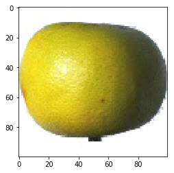
At the current time, we are able to read the dataset content, access the class folders within its Training and Test directories, access individual images within each class, and reading them as NumPy arrays. If we are to read all images within a class in a single NumPy array, then it can be simply created according to the following steps:
The above steps are implemented below. The if statement exactly after the for loop checks that the image file is a JPG file.
import numpy
import keras
import os

train_dir_content = os.listdir("/root/.keras/datasets/fruits-360/Training")

print("Number of Classes :", len(train_dir_content))

current_class_name = train_dir_content[0]
class_dir = os.path.join("/root/.keras/datasets/fruits-360/Training", current_class_name)
images_in_class = os.listdir(class_dir)

print("Number of Samples in Class Named", current_class_name, ":" , len(images_in_class))

dataset_array = []
for image_file in images_in_class:
    if image_file.endswith(".jpg"):
      image_file_dir = os.path.join(class_dir, image_file)

      img = keras.preprocessing.image.load_img(image_file_dir)
      img_array = keras.preprocessing.image.img_to_array(img)

      img_array = img_array/255.0
      dataset_array.append(img_array)

dataset_array = numpy.array(dataset_array)
print("Class", current_class_name," Array Shape :", dataset_array.shape)
The result of the print statements is given below.
Number of Classes : 102
Number of Samples in Class Named Pomelo Sweetie : 450
Class Pomelo Sweetie Array Shape : (450, 100, 100, 3)
The above code reads all images within the first class and adds them to a single NumPy array named dataset_array. Because there are 450 images in the class and each image shape is (100, 100, 3), the shape of the dataset_array is (450, 100, 100, 3).
The previous section discussed processing all images in just a single class. We can extend it to work with all classes either the Training or the Test folders. This is by using another loop that loops through the classes within such folders.
After the first step in the previously listed 5 steps, a new step will be added to loop though the class directories. The new list as given below. By doing this, we can read all training and testing images in the dataset.
The code that reads all images within the Training folder is listed below.
import numpy
import keras
import os

train_dir_content = os.listdir("/root/.keras/datasets/fruits-360/Training")

print("Number of Classes :", len(train_dir_content))

dataset_array = []

for current_class_name in train_dir_content:

    class_dir = os.path.join("/root/.keras/datasets/fruits-360/Training", current_class_name)
    images_in_class = os.listdir(class_dir)

    print("Number of Samples in Class Named", current_class_name, ":", len(images_in_class))

    for image_file in images_in_class:
        if image_file.endswith(".jpg"):
            image_file_dir = os.path.join(class_dir, image_file)

            img = keras.preprocessing.image.load_img(image_file_dir)
            img_array = keras.preprocessing.image.img_to_array(img)

            img_array = img_array / 255.0
            dataset_array.append(img_array)

dataset_array = numpy.array(dataset_array)
print("Training Data Array Shape :", dataset_array.shape)
After the code completes successfully, the shape of the NumPy array is printed as given below.
Training Data Array Shape : (52718, 100, 100, 3)The previous code uses the Training directory in reading the images. If the name of the train data directory, which is Training, is replaced by the name of the test data directory, which is Test, then the above code can work with the test data. The modified code is listed below. Otherwise replacing Training by Test, everything is identical to the previous code.
import numpy
import keras
import os

train_dir_content = os.listdir("/root/.keras/datasets/fruits-360/Test")

print("Number of Classes :", len(train_dir_content))

dataset_array = []

for current_class_name in train_dir_content:

    class_dir = os.path.join("/root/.keras/datasets/fruits-360/Test", current_class_name)
    images_in_class = os.listdir(class_dir)

    print("Number of Samples in Class Named", current_class_name, ":" , len(images_in_class))

    for image_file in images_in_class:
        if image_file.endswith(".jpg"):
          image_file_dir = os.path.join(class_dir, image_file)

          img = keras.preprocessing.image.load_img(image_file_dir)
          img_array = keras.preprocessing.image.img_to_array(img)

          img_array = img_array/255.0
          dataset_array.append(img_array)

dataset_array = numpy.array(dataset_array)
print("Test Data Array Shape :", dataset_array.shape)
At the end of the code, the size of the NumPy array holding all test data is printed as given below. The array has 17692 elements, which is the number of test samples across all classes) and the shape of each one of them is (100, 100, 3).
Test Data Array Shape : (17692, 100, 100, 3)Up to this time, there are 2 different codes for working with the train and test data despite being identical except for specifying the path to work on. We can build a single function that accepts the path and returns the NumPy array for all images in all classes within it. The function is named images_to_array() and its code is listed below.
import numpy
import keras
import os

def images_to_array(dataset_dir, image_size):
    dataset_array = []
    dataset_labels = []

    class_counter = 0

    classes_names = os.listdir(dataset_dir)
    for current_class_name in classes_names:
        class_dir = os.path.join(dataset_dir, current_class_name)
        images_in_class = os.listdir(class_dir)

        print("Class index", class_counter, ", ", current_class_name, ":" , len(images_in_class))

        for image_file in images_in_class:
            if image_file.endswith(".jpg"):
              image_file_dir = os.path.join(class_dir, image_file)

              img = keras.preprocessing.image.load_img(image_file_dir, target_size=(image_size, image_size))
              img_array = keras.preprocessing.image.img_to_array(img)

              img_array = img_array/255.0

              dataset_array.append(img_array)
              dataset_labels.append(class_counter)
        class_counter = class_counter + 1
    dataset_array = numpy.array(dataset_array)
    dataset_labels = numpy.array(dataset_labels)
    return dataset_array, dataset_labels
The images_to_array() function accepts 2 arguments:
It is normal to have the data path as an argument but why passing the image size? The reason is that the MobileNet only works with pre-defined sizes of the input images. The dataset being handled must have its image size identical to the size expected by the MobileNet. Otherwise, an error will occur. Because the image size accepted by the MobileNet has the number of rows equal to the number of columns, then just a single value is passed to the image_size argument. When reading the image using the load_image() function in Keras, the target_size argument resizes the image automatically in the same step.
By calling the images_to_array() function with the proper path, the images in that path and its child folders will be read and added to the NumPy array which will be returned by the function. In addition to the array that holds the images, there is another array named dataset_labels which holds the labels of the dataset. There is a variable named class_counter which is initialized to 0 and increments for each class. All images within the same class are given the same label which is added to that dataset_labels array.
According to the next code, the dataset is firstly downloaded according to the link we got and the directory of the dataset is saved in the base_dir variable.
After that, the train data directory is prepared in the train_dir variable. The second one calls the images_to_array() function after passing the train data directory and the image size which is 128. Why 128? Let's explain.
MobileNet accepts 4 image sizes which are 224, 192, 160, and 128. Remember that the image size for the Fruits360 dataset is 100x100. From the 4 sizes, 128 is the nearest and thus it is the used one. The image shape now will be (128, 128, 3).
The third one prints the shape of the returned array by such function. To avoid rerunning the code each time the dataset array is needed, the fourth and fifth lines save the NumPy arrays in .npy files in the root directory for later use. This is for the test data.
import numpy
import os
import tensorflow as tf

zip_file = tf.keras.utils.get_file(origin="https://storage.apis.com/kaggle-datasets/5857/414958/fruits-360_dataset.zip?AccessId=web-data@kaggle-161607.iam.gserviceaccount.com&Expires=1566314394&Signature=rqm4aS%2FIxgWrNSJ84ccMfQGpjJzZ7gZ9WmsKok6quQMyKin14vJyHBMSjqXSHR%2B6isrN2POYfwXqAgibIkeAy%2FcB2OIrxTsBtCmKUQKuzqdGMnXiLUiSKw0XgKUfvYOTC%2F0gdWMv%2B2xMLMjZQ3CYwUHNnPoDRPm9GopyyA6kZO%2B0UpwB59uwhADNiDNdVgD3GPMVleo4hPdOBVHpaWl%2F%2B%2BPDkOmQdlcH6b%2F983JHaktssmnCu8f0LVeQjzZY96d24O4H85x8wdZtmkHZCoFiIgCCMU%2BKMMBAbTL66QiUUB%2FW%2FpULPlpzN9sBBUR2yydB3CUwqLmSjAcwz3wQ%2FpIhzg%3D%3D",
                                   fname="fruits-360.zip", extract=True)
base_dir, _ = os.path.splitext(zip_file)

train_dir = "/root/.keras/datasets/fruits-360/Training"
image_size = 128
train_dataset_array, train_dataset_array_labels = images_to_array(dataset_dir=train_dir, image_size=image_size)
print("Training Data Array Shape :", train_dataset_array.shape)
numpy.save("train_dataset_array.npy", train_dataset_array)
numpy.save("train_dataset_array_labels.npy", train_dataset_array_labels)
For the test data, the same happens except for passing the directory of the test data.
import numpy
import os
import tensorflow as tf

zip_file = tf.keras.utils.get_file(origin="https://storage.apis.com/kaggle-datasets/5857/414958/fruits-360_dataset.zip?AccessId=web-data@kaggle-161607.iam.gserviceaccount.com&Expires=1566314394&Signature=rqm4aS%2FIxgWrNSJ84ccMfQGpjJzZ7gZ9WmsKok6quQMyKin14vJyHBMSjqXSHR%2B6isrN2POYfwXqAgibIkeAy%2FcB2OIrxTsBtCmKUQKuzqdGMnXiLUiSKw0XgKUfvYOTC%2F0gdWMv%2B2xMLMjZQ3CYwUHNnPoDRPm9GopyyA6kZO%2B0UpwB59uwhADNiDNdVgD3GPMVleo4hPdOBVHpaWl%2F%2B%2BPDkOmQdlcH6b%2F983JHaktssmnCu8f0LVeQjzZY96d24O4H85x8wdZtmkHZCoFiIgCCMU%2BKMMBAbTL66QiUUB%2FW%2FpULPlpzN9sBBUR2yydB3CUwqLmSjAcwz3wQ%2FpIhzg%3D%3D",
                                   fname="fruits-360.zip", extract=True)
base_dir, _ = os.path.splitext(zip_file)

test_dir = "/root/.keras/datasets/fruits-360/Test"
image_size = 128
test_dataset_array, test_dataset_array_labels = images_to_array(dataset_dir=test_dir, image_size=image_size)
print("Test Data Array Shape :", test_dataset_array.shape)
numpy.save("test_dataset_array.npy", test_dataset_array)
numpy.save("test_dataset_array_labels.npy", test_dataset_array_labels)This tutorial introduced used Keras for building NumPy arrays that holds all images in the Fruits360 dataset in addition to their class labels.
The downloaded dataset will be fed later to the MobileNet model for transfer learning. After the model learns how to work with the Fruits360 dataset, it will be saved. The NumPy arrays prepared in this tutorial will be fed to the saved model for extracting features. The extracted features will also be saved for later use for training the artificial neural network.
Part 1: Image Classification using Features Extracted by Transfer Learning in Keras
Part 3: Image Classification using Features Extracted by Transfer Learning in Keras
Ahmed Gad - August 26, 2019
Ahmed Gad - August 26, 2019
Ahmed Gad - August 26, 2019
Alibaba F(x) Team - June 20, 2022
Alibaba F(x) Team - February 23, 2021
Alibaba Clouder - September 2, 2019
 Platform For AI
A platform that provides enterprise-level data modeling services based on machine learning algorithms to quickly meet your needs for data-driven operations.
Learn More Epidemic Prediction Solution
This technology can be used to predict the spread of COVID-19 and help decision makers evaluate the impact of various prevention and control measures on the development of the epidemic.
Learn More Container Compute Service (ACS)
A cloud computing service that provides container compute resources that comply with the container specifications of Kubernetes
Learn More Online Education Solution
This solution enables you to rapidly build cost-effective platforms to bring the best education to the world anytime and anywhere.
Learn More