Join Reorder is a widely recognized and highly important problem in the field of database optimization. Its objective is to determine the optimal sequence in which tables are joined in an SQL statement to achieve the best query performance. Different databases employ different algorithms for Join Reorder. This article provides an overview of the implementation methods, advantages, and disadvantages of Join Reorder in various popular databases. Additionally, it introduces the Join Reorder implementation algorithm based on rule transformation in Alibaba Cloud PolarDB for Xscale (PolarDB-X) and the underlying principles behind it.
PolarDB-X is a high-performance cloud-native distributed database service developed by Alibaba Cloud. It offers features such as high throughput, large storage capacity, low latency, scalability, and high availability in the cloud era.
Let's take TPCH Q9 as an example to illustrate the basic concept of Join Reorder. It is an SQL statement that joins six tables.
SELECT nation,
       o_year,
       sum(amount) AS sum_profit
FROM
  (SELECT n_name AS nation,
          extract(YEAR
                  FROM o_orderdate) AS o_year,
          l_extendedprice * (1 - l_discount) - ps_supplycost * l_quantity AS amount
   FROM part,
        supplier,
        lineitem,
        partsupp,
        orders,
        nation
   WHERE s_suppkey = l_suppkey
     AND ps_suppkey = l_suppkey
     AND ps_partkey = l_partkey
     AND p_partkey = l_partkey
     AND o_orderkey = l_orderkey
     AND s_nationkey = n_nationkey
     AND p_name LIKE '%green%') AS profit
GROUP BY nation,
         o_year
ORDER BY nation,
         o_year DESC;
Query graph is an undirected graph, in which each node on the graph represents each table, and the edge between the nodes represents a Join between two tables. In general, an SQL query that joins multiple tables can be classified into Chain Join, Star Join, and Full Join based on the shape of the query graph. The query graph of TPCH Q9 is as follows:
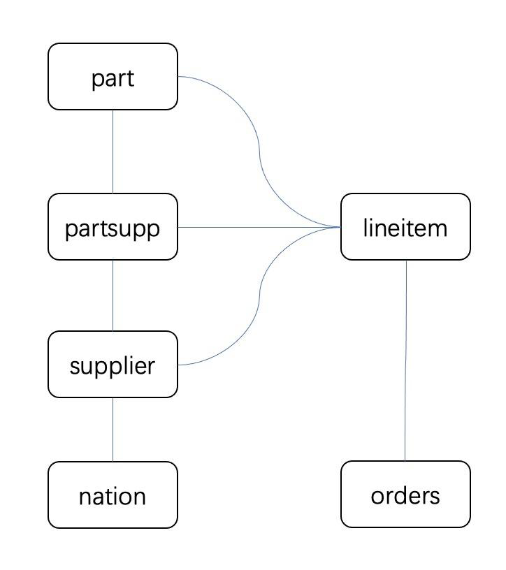
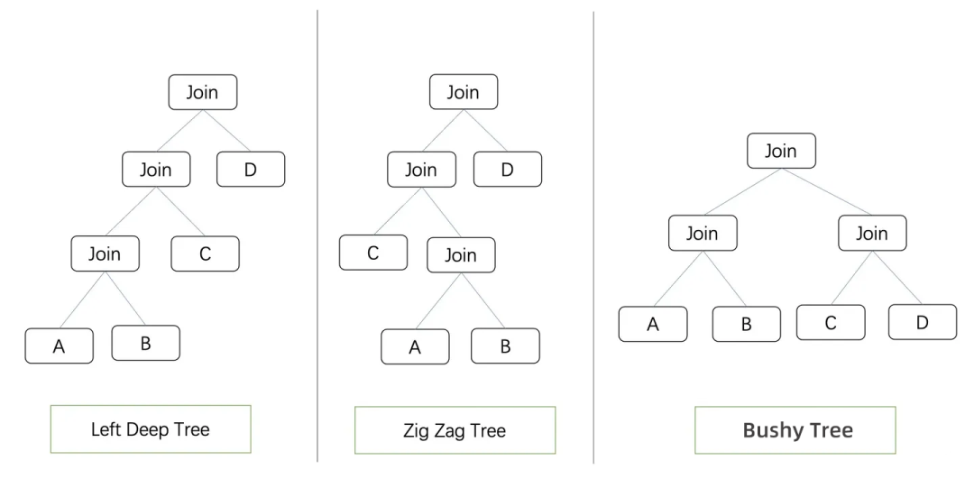
In general, databases typically implement Join algorithms with only two inputs. A Join Tree is a binary tree where leaf nodes represent tables to be joined, and non-leaf nodes represent Join operators. Depending on the shape of the Join Tree, it can be classified as Left Deep Tree, ZigZag Tree, or Bushy Tree.
The Left Deep Tree restricts the right side of the Join node to only a leaf node. Many databases use the left deep tree as the search space for Join Reorder by default. The ZigZag Tree is an extension of the left deep tree, allowing for swapping of left and right nodes. The Bushy Tree offers the most flexible structure, allowing tables to be joined in any order.
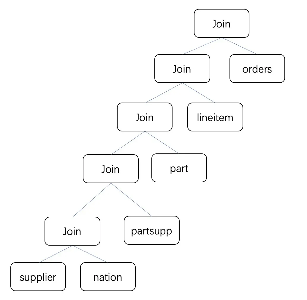
Different Join Reorder algorithms generate different join trees. The Join Trees describe the order in which each table joins. One possible Join Tree shape for TPCH Q9 is as follows:
The Join Cardinality represents the size of the intermediate result set produced by the Join operator. It serves as a crucial factor for all Join Reorder algorithms to determine the order of execution. In general, a smaller intermediate result set generated by a Join operator leads to better performance in subsequent Joins.
Estimating the size of a single table is relatively straightforward. It can be approximated based on the number of rows in the table and the average row length. If a table has filter conditions, methods such as histograms or sketches can be used to estimate the number of filtered rows.
The following formula is commonly used to estimate the number of rows in the intermediate result set of a Join operation:
LeftRowCount * RightRowCount / MAX(LeftCardinality, RightCardinality)LeftRowCount and RightRowCount respectively represent the number of input rows in the left and right columns of the Join, and LeftCardinality represent the NDV (Number Of Distinct Value) of the input rows in the left column of the Join. This is true of RightCardinality. Specifically, the number of rows of a Cross Join without a Join condition is LeftRowCount * RightRowCount.
In the implementation of databases, different Join algorithms often have multiple implementations. Common Join algorithms in various scenarios include NestedLoop Join, Index NestedLoop Join, Hash Join, and Sort Merge Join. Each Join algorithm has its associated costs. Take the CPU cost as an example:
The execution cost of Hash Join
CPU cost= Probe weight * Probe data volume + Build weight * Build data volumeThe execution cost of Nested Loop Join execution
CPU cost= Join weight × Left data volume × Right data volumeThe execution cost of Sort Merge Join
CPU cost=Left input data sorting cost + Right input data sorting cost + Merge costCommon Join Reorder algorithms can be divided into:
Generally, databases use these two types of algorithms to balance the optimization time and search space size based on the number of Joins.
The algorithm uses a greedy approach to select the table that minimizes the output RowCount of the current Join when joining from one table to N tables. The selected table sequence is used to construct a left deep tree. [1]
Algorithm process: The search space is left deep tree. Assume that N tables are input. Build a complete JoinOrder from one table to N tables.
One disadvantage of this algorithm is that greedily selecting the first table has a significant impact on the entire Join Order, making it prone to getting trapped in a locally optimal solution.
The greedy heuristic Join Reorder algorithm for multiple sequences [1]: (The algorithm supports SemiJoin and Outer Join. For the conciseness of the algorithm, only InnerJoin is considered) Idea can heuristically generate N Join orders for the input N tables (the first table of each sequence is different) and construct a left deep tree. Then compare the Cost of N Join orders and choose the best one.
For example, when N=5, five orders are heuristically generated, and the one with the lowest cost is selected: [1,4,5,2,3] [2,5,1,3,4] [3,1,5,2,4] [4,5,3,1,4] [5,3,2,1,4].
Algorithm process: Assuming the input is an inner join of N tables,
1. Set the weighti for the i-th and j-th tables, where greater weight indicates an earlier join between the two tables.
Weighti = 3, i and j have equivalent join conditions.
Weighti = 2, i and j have non-equivalent join conditions (>, >=, <, <=, !=).
Weighti = 1, other cases (i and j may be Cartesian sets)
2. Assume that the first table of the sequence is X, and the selection rules of the second table Y are as follows.
3. Give priority to Y with large weight [X] [Y]
4. If the weight values are equal, the Cardinality value of the column corresponding to the Join condition of Y in Y Join X is considered. The larger the Cardinality value, the higher the priority. (Note: Higher cardinality means a smaller result set for the Join.)
5. The selection of the K-th table follows a similar process.
6. Use the final N tables to construct the left deep tree according to the above selection sequence.
7. Choose the Join order with the lowest cost
It's important to note that the Greedy Heuristic Join Reorder algorithm for multiple sequences considers multiple Join sequences and selects the sequence with the lowest cost. The cost can be any custom-defined cost.
Systems such as Flink and Drill utilize this Join Reorder algorithm.
GOO(Greedy Operator Ordering)[1]
● For the above scenario where greedy heuristic algorithm can only construct left deep trees, GOO can construct BushyTree
● Greedy heuristic algorithm only considers joining JoinTree and a table, while GOO algorithm considers joining JoinTree and JoinTree.
Algorithm process: Assume that N tables are input and make T equals to the set of N tables:
1. while |T| > 1
a) find two JoinTrees in T, T[i] and T[j], to minimize their Join result set.
b) T = (T T[i] T[j]) c. T = T U {T[i] join T[j]}
2. The only element in the final T is the JoinOrder searched greedily in the Bushy Tree space.
PostgreSQL uses GEQO algorithm when the number of tables is large (be equal or greater than 12). Assume that N tables are input:
By simulating genetic inheritance, the algorithm selects a paternal and maternal chromosome, exchanges fragments, and generates a child chromosome. It eliminates suboptimal chromosomes and iterates among the excellent chromosomes for several generations to obtain an optimal order.
Algorithm process: Assuming the input consists of N tables, the initial chromosome pool size is set to PoolSize, and the number of chromosome iterations is set to generations (default is 2^(N-1)).
One disadvantage of the genetic algorithm is that each execution plan result can vary, leading to unstable performance. This can be problematic in scenarios that require stable performance for each query result.
The MySQL database has been around for more than twenty years. As an OLTP-oriented database, its Join Reorder is a Left Deep Tree enumeration algorithm. The Join Reorder considers using the Index NestedLoop Join.
Algorithm Process
The Join Reorder algorithm for Bottom-Up enumeration uses dynamic planning techniques to avoid repeated calculations of intermediate results and enumerate the Bushy Tree space.
The following uses the concept of CCP (csg-cmp-pair) to describe the algorithm [3].
Assume that N tables are input and the query graph is connected. Define CCP(S1, S2) for the set S of N tables:
We can find the best plan step by step by explicitly traversing the CCP from table 1 to table N.
PS: The number of CCP is related to the shape of the query graph. For example, the number of CCP in a full query graph is larger than that in a star query graph, and the number of CCP in a chain query graph is the smallest.
Algorithm Process
The Join Reorder algorithm for Bottom-Up enumeration can effectively deal with the problem of Bushy Tree space enumeration, and can use dynamic planning to solve the problem of repeated calculation of intermediate results. This algorithm can only handle the specific kind of problems of Join Reorder. If you want to add more optimization to the Join Reorder process to obtain the global optimal solution, such as transpose Agg and Join, this algorithm cannot do it.
The Join Reorder algorithm based on rule transformation requires the implementation with the assistance of the Top-Down Cascades optimization framework [4].
Join Reorder is achieved by utilizing a set of Join transformation rules. The planning space search engine applies these Join rules until the dynamic planning solution is completed. This process involves traversing the Join (sequential) space corresponding to each rule. It can be observed that a set of Join Reorder rules corresponds to a specific Join space, and different Join Reorder rules correspond to different Join spaces.
The Join Reorder rules support various types of Join reorder, including Inner, Outer, Semi, and Anti Joins. These Join Reorder rules have been summarized in a paper [5]6. In the figure, 'e' represents a table, 'a' and 'b' represent a Join, while 'p' represents Join conditions. The table below describes the scenarios in which two different types of Joins can be transformed (assoc, l-asscom, r-asscom). Additionally, there is a Join commutative law (comm) that is only applicable to Inner Joins, allowing the exchange of the left and right tables.
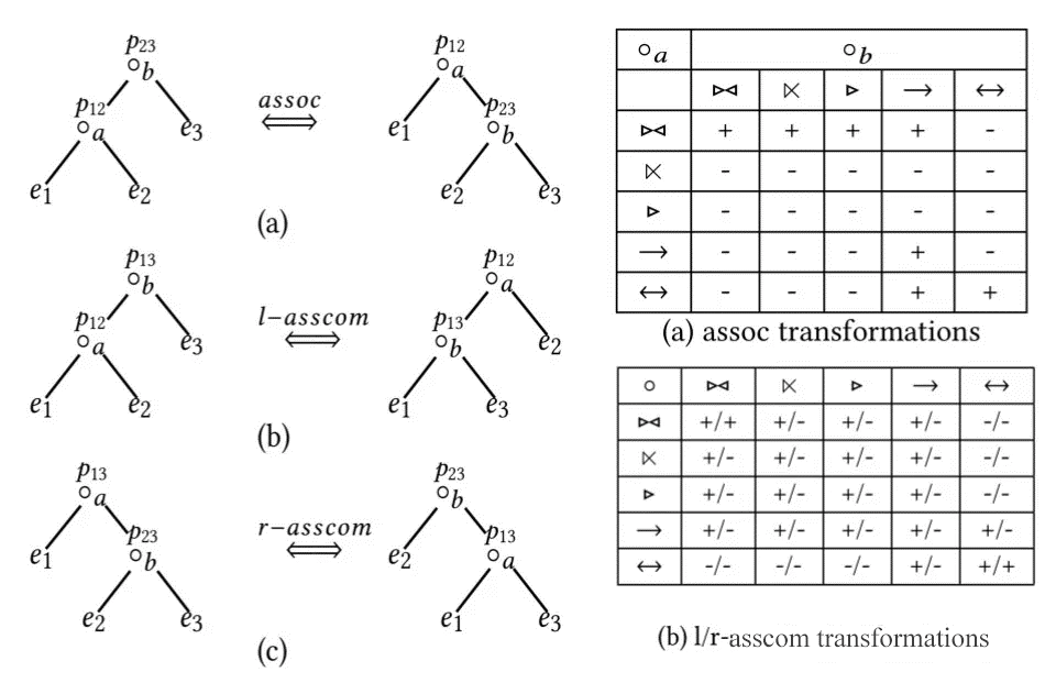
Different rule sets correspond to different search spaces:
Left Deep Tree: bottom comm rule: a ⨝ B→B ⨝ A, only applied to the l-asscom rule of the bottom two tables of the left deep tree: (a ⨝ b) ⨝ C→ (a ⨝ c) ⨝ b
Zig-Zag Tree: comm rule: ⨝ A B→B ⨝ A l-asscom rule: (A ⨝ B) ⨝ C→ (A ⨝ C) ⨝ B
Bushy Tree: comm rule: A ⨝ B→B ⨝ A assoc rule: (A ⨝ B) ⨝ C→A ⨝ (B ⨝ C)
Intuitively, the search space of the entire Bushy Tree can be enumerated by applying the commutative and associative laws.
The advantage of this algorithm is its ability to utilize Branch and Bound for space pruning during the Top-Down dynamic planning process of the Cascades engine. Additionally, it efficiently handles the Interesting Order problems using a physical property-driven search approach. By incorporating the optimization rules of Join Reorder and other types into the Cascades search engine, it is possible to obtain the global optimal solution.
Databases such as SQL Server, CockroachDB, and PolarDB Distributed Edition employ these types of algorithms.
The Join Reorder algorithm used by PolarDB distributed edition is a Top-Down Join Reorder algorithm based on rule transformation.
PolarDB Distributed Edition will use the duplicate-free Join Reorder rules 7 to improve optimization efficiency. Duplicate-Free rule indicates that this set of rules will not generate duplicates and can traverse the same complete space. The core idea is to avoid generating duplicates by recording the "historical path information" of operator conversion.
The set of duplicate-free rules for two spaces is as follows:
Left Deep Tree: Rule1 (l-asscom) : (A ⨝ 0B) ⨝ 1C → (A ⨝ 2C) ⨝ 3B , Rule1 cannot act on ⨝ 3 Rule2 (comm) again : A ⨝ 0B → B ⨝ 1A,Rule2 cannot act on ⨝ 1 again
Bushy Tree: Rule1 (comm): A ⨝ 0B→B ⨝ 1A, Rule1, 2, 3, 4 do not act on ⨝ 1 Rule2 (r-assoc) again: (A ⨝ 0B) ⨝ 1C →A ⨝ 2(B ⨝ 3C), Rule2, 3, 4 do not act on ⨝ 2 Rule3 (l-assoc) again: A ⨝ 0(B ⨝ 1C) → (A ⨝ 2B) ⨝ 3C , Rule2, 3, 4 do not act on⨝ 3 Rule4 (exchange) again: (A ⨝ 0B) ⨝ 1(C ⨝ 2D) → (A ⨝ 3C) ⨝ 4(B ⨝ 5D) , Rule1, 2, 3, 4 do not act on⨝ 4 again
As you can see, the duplicate-free rule becomes complicated because it records "historical path information". The information is actually encoded in the Join operators, so the corresponding information is changed each time the Join operator is converted. Additional conditions also need to be checked for each rule matching. Zig-Zag Tree can give similar ideas for Left Deep Tree.
Search space size: Bushy Tree > Zig-Zag Tree > Left Deep Tree
The larger the search space is or the more Joins are, the longer the optimization search time is. To keep the optimization time within a certain period of time, PolarDB distributed edition uses the Adaptive Search Space to determine the size of the search space based on the purpose of the Join.
| Number of tables | Search space |
| <= 4 | Bushy Tree |
| <= 6 | Zig-Zag Tree |
| <= 8 | Left Deep Tree |
| >=9 | Heuristic |
When the number of tables is greater than or equal to 9, the PolarDB-X uses the greedy heuristic Join Reorder algorithm for multiple sequences to accelerate the Join Reorder process.
In PolarDB distributed edition, Join Reorder rules and other key optimization rules will form a larger search space to obtain the global optimal solution.
Join algorithm rules: The sequence of Joins is closely related to the specific Join operator physical algorithm because different Join operator physical algorithms have different costs. PolarDB distributed edition supports HashJoin, Sort Merge Join, NestedLoop Join, and BKA Join (distributed Index Nested Join). Join algorithm rules and Join Reorder rules together form a search space.
Join pushdown rules: The PolarDB distributed edition supports Join pushdown. Therefore, the Join pushdown rules and Join Reorder rules together form a search space.
Agg and Join exchange rules: The exchange between Agg and Join can greatly reduce the [9] data volume processed by Join, so this rule will also form a search space together with the Join Reorder rule.
Index selection rules: PolarDB distributed edition supports global secondary indexes. Different global secondary indexes will affect Join pushdown and Join algorithm rules. Therefore, this rule also forms a search space with the Join Reorder rules.
Space pruning is a great feature of Top-Down dynamic planning. It ensures that the pruned space can also find the optimal solution. This is an important advantage over Bottom-Up dynamic planning. Take the three-table Join as an example to see how to prune space.
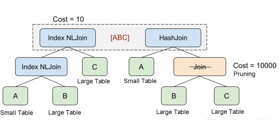
If the ABC table Join is optimized according to the initial order, tables A, B and C use Index Nested Loop Join in turn and the cost value is calculated as 10. Then B Join C is constructed through Join Reorder rules. However, we see that the minimum cost of B Join C is 1000 because two large tables are joined. Since there is already an execution plan with a cost of 10 in the [ABC] equivalent set, then you can directly cut out [BC] and no longer generate physical execution plans for them, because no matter what physical execution plan they choose, the cost will never be lower than 10. This is the Branch And Bound space pruning.
The application order of the rules here shows that if the physical transformation rules are applied from top to bottom, then we have the opportunity to prune without searching part of the space. In general, search engines are guided by specific heuristics to apply physical transformation rules to find a low-cost execution plan as soon as possible, and use its cost to prune space.
This article summarizes common Join Reorder algorithms in the database field, including:
| Join Reorder algorithm | Default database | INFO |
| Greedy Heuristic Join Reorder Algorithm for Single Sequence | TiDB | Left Deep Tree |
| Greedy Heuristic Join Reorder Algorithm for Multiple Sequences | Flink, Drill, and PolarDB distributed edition | Left Deep Tree , you can compare N Join sequences and select the one with the lower cost. |
| Genetic Algorithm | PostgreSQL | This feature is enabled only when the number of tables is greater than 12. The Join sequence is unstable each time. |
| Join Reorder Algorithm for Depth-First Enumeration | MySQL | Left Deep Tree , when the number of tables is less than or equal to 7, the algorithm complexity is N! and dynamic planning is not used. |
| Join Reorder Algorithm for Bottom-Up Enumeration | PostgreSQL | Bottom-Up dynamic planning enumeration of Left Deep Tree or Bushy Join Tree search space |
| Join Reorder Algorithm for Top-Down Enumeration Based on Rule Transformation | PolarDB distributed edition, SQLServer, and CockroachDB | Top-Down dynamic planning enumeration of Left Deep Tree or Bushy Join Tree, which can be used for space pruning and mixed with other optimization rules for global optimization. |
In PolarDB distributed edition, the greedy Join Reorder algorithm for multiple sequences is used when the number of tables is large (greater than or equal to 9).
On the other hand, when the number of tables is small (less than 9), PolarDB distributed edition employs the Top-Down Join Reorder algorithm based on rule transformation. This algorithm offers several advantages:
● Use the duplicate-free Join Reorder rules to improve the efficiency of Reorder operations.
● Use Adaptive Search Space to control the search space size.
● Use Join Reorder rules, Join algorithm rules, Join pushdown rules, Agg and Join exchange rules, and index selection rules to build a search space to obtain the global optimal solution.
● Use Top-Down search for space pruning.
Check Out Free Tier & Special Offers of Alibaba Cloud Database Products: https://www.alibabacloud.com/product/databases
[1] https://db.in.tum.de/teaching/ws1415/queryopt/chapter3.pdf
[2] https://www.postgresql.org/docs/9.1/geqo-pg-intro.html
[3] Analysis of Two Existing and One New Dynamic Programming Algorithm for the Generation of Optimal Bushy Join Trees without Cross Products
[4] The Cascades Framework for Query Optimization
[5] On the Correct and Complete Enumeration of the Core Search Space
[6] Improving Join Reorderability with Compensation Operators
[7] The Complexity of Transformation-Based Join Enumeration
[8] Measuring the Complexity of Join Enumeration in Query Optimization
[9] eager aggregation and lazy aggregation
[Infographic] Highlights | Database New Feature in September 2023
About Database Kernel | Deep Analysis on the Optimization and Evolution of PolarDB DDL Locks
ApsaraDB - August 7, 2023
ApsaraDB - September 29, 2021
ApsaraDB - December 25, 2024
ApsaraDB - November 8, 2024
ApsaraDB - November 18, 2025
Alibaba EMR - May 20, 2022
 PolarDB for Xscale
Alibaba Cloud PolarDB for Xscale (PolarDB-X) is a cloud-native high-performance distributed database service independently developed by Alibaba Cloud.
Learn More PolarDB for PostgreSQL
Alibaba Cloud PolarDB for PostgreSQL is an in-house relational database service 100% compatible with PostgreSQL and highly compatible with the Oracle syntax.
Learn More PolarDB for MySQL
Alibaba Cloud PolarDB for MySQL is a cloud-native relational database service 100% compatible with MySQL.
Learn More LedgerDB
A ledger database that provides powerful data audit capabilities.
Learn MoreMore Posts by ApsaraDB