By Yiwei Yao
In the era of generative AI, there has been a surge in the development of vector databases. Many people believe that the only difference between a vector database and a traditional database is the addition of a vector index. However, as the application of large models expands to core business areas, combining large models, vector indexes, and structured data analysis results through complex code engineering hinders large-scale replication. Concurrent query performance, data consistency, high reliability, and auto scaling become increasingly important. To address the intelligent upgrade requirements of enterprise data architecture in the next five years, Alibaba Cloud AnalyticDB has developed an enterprise-level vector database. It is the only vector engine recommended by OpenAI and LangChain among domestic cloud vendors. In this article, we will explore the insightful speech delivered by Yiwei Yao, the technical director of Alibaba Cloud AnalyticDB, at the 2023 QCon Global Software Development Conference (Beijing Station). Mr. Yao reveals the core technology of AnalyticDB's fully in-house enterprise-level vector database and the technological evolution roadmap of the new generation of vector databases in terms of cloud-native compute-storage separation and native AI.
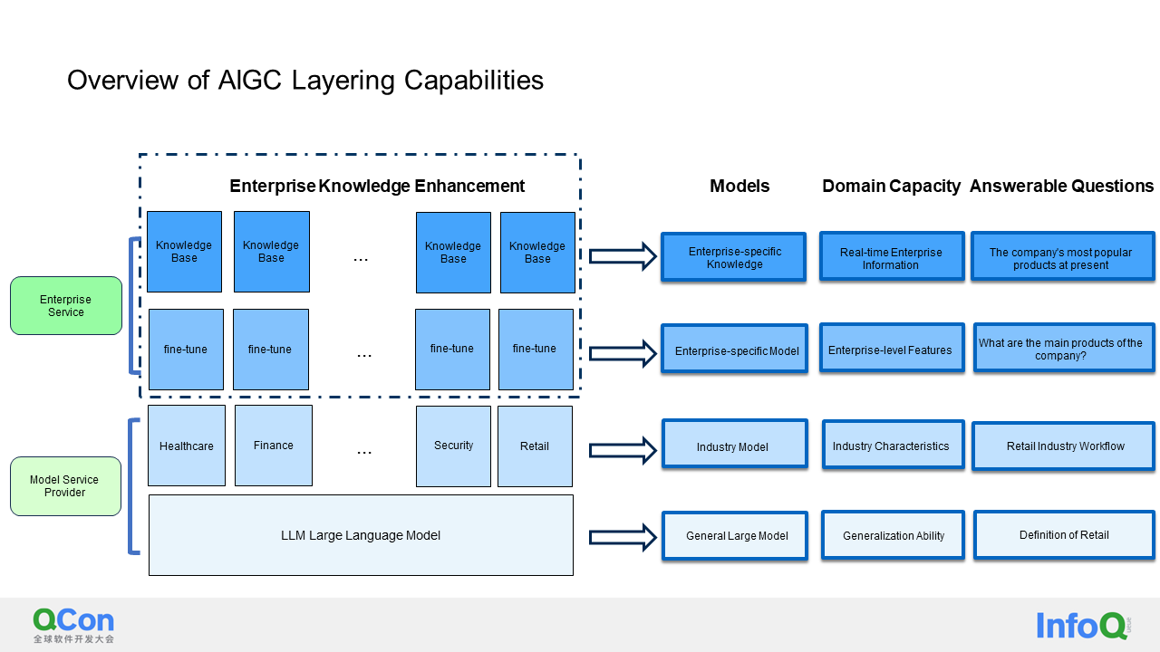
In the era of generative AI, what role do vector databases play for enterprises? Let's first examine the layers of vector databases and LLM (large language models). At the bottom layer, we have a general large language model that can answer common questions. For example, if you ask it to define "retail," it can provide a clear answer.
The layer above is the industry model, which is a customized large language model tailored specifically for different industries. For instance, it can be customized for the financial, security, or retail industries, and specific industry knowledge is used to enhance its training. The industry model can answer questions regarding specific workflows in the retail industry accurately, which goes beyond the capabilities of a regular large language model. Above the industry model is the enterprise private model, which also consists of two layers. The first layer is the enterprise-specific model, fine-tuned by the enterprise based on the industry model and its own proprietary internal knowledge. It can answer questions like the main products of the company. However, fine-tuning is costly and time-consuming, which explains why enterprises do not perform it frequently.
In the context of the big data explosion, where enterprise data knowledge continuously flows in, we need the fourth layer - a dedicated knowledge base for enterprises, usually implemented through vector databases. This knowledge base can answer questions like the most searched product of our company in the last three days or the most popular product recently. It provides real-time information. In many cases, the vector database layer can also correct the illusion of large language models.
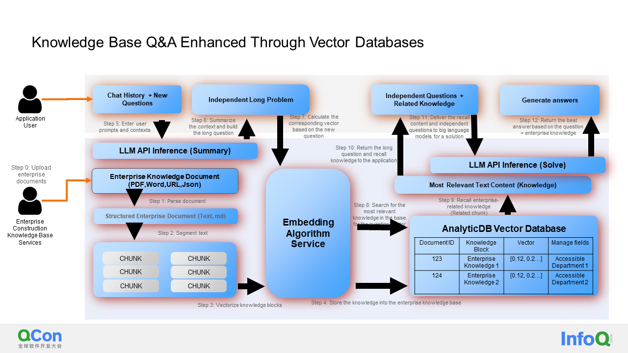
I will give a specific example to explain how we utilize a vector database and a language model to implement an intelligent Q&A service in the scenario of vector database enhancement.
Let's first focus on the following section, which illustrates the entire data import process: parsing documents, segmenting the document, generating embeddings using the Embedding algorithm, and storing the original content and vectors obtained through the Embedding algorithm in the vector database.
During the search process, as it may involve multiple rounds of conversation, I will provide the previous chat record and the new question to the Language Model (LLM). LLM will then provide a summarized, independent long question. Subsequently, I will perform embedding on this long question and search in the vector database. In this case, we can search and retrieve the most relevant knowledge chunk to this question in real-time. I will then deliver the knowledge chunk and an independent question to LLM (knowledge chunks are usually combined with independent questions in the form of a prompt). At this point, LLM can provide an answer that incorporates the real-time knowledge stored in the vector database.
Next, let's explore how we can implement a vector database. Firstly, I would like to introduce some fundamental concepts. What exactly does a vector database do? Essentially, it aims to search for the k vectors nearest to a given vector. The definition of proximity can be based on inner product, Euclidean distance, or cosine distance. Along with the definition of distance, we also need to define vector search algorithms.
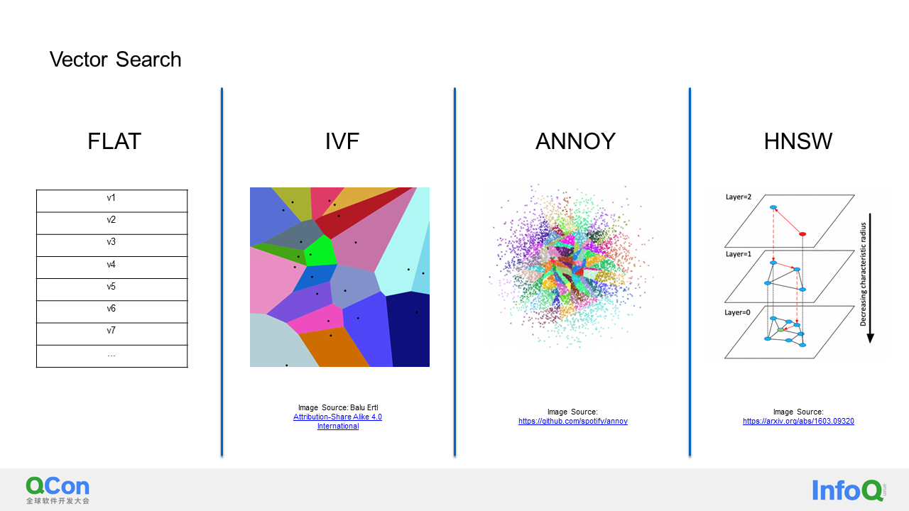
Vector search algorithms can generally be divided into two categories. The first category is accurate search, such as FLAT, which retrieves vectors one by one and selects the top k. While this approach achieves a high recall rate, its execution performance is relatively lower due to the need for global scanning. The well-known KD tree also falls into this category, allowing you to find the most accurate top k, which is part of the KNN algorithm.
The second category is Approximate Nearest Neighbor (ANN). Algorithms in this category may not provide the most accurate top k vectors, but they offer higher execution efficiency.
For example, IVF groups all vectors into a vector space, where the K-means algorithm can be utilized to find center points. You can then assign each vector to its closest center point. During the search, you only need to find the corresponding center point and search for the top k vectors within it. However, there may be cases where the nearest points are not within the space of the center points found using the K-means algorithm. In such situations, additional adjacent spaces need to be explored. The general idea is as follows.
Apart from IVF, there is another type of tree-based algorithm in the ANN category, such as the ANNOY algorithm proposed by Spotify. This algorithm is similar to IVF, where the space is continuously divided until reaching the leaf node of the last layer of the tree. The construction process stops when the number of vectors is less than k. Tree-based algorithms also face the same problem as IVF, where the leaf nodes found may not contain the required top k nodes during the search. In such cases, methods like adding priority queues and building additional trees can be employed to achieve a higher recall rate.
The last type of ANN is the graph algorithm, which includes the well-known NSW algorithm and HNSW algorithm. HNSW is essentially a combination of multiple NSWs. I will provide a detailed explanation of HNSW because our tests have shown that HNSW performs excellently in terms of execution efficiency and recall rate for high-dimensional vectors. As a result, we have chosen HNSW as the default vector search algorithm for AnalyticDB.
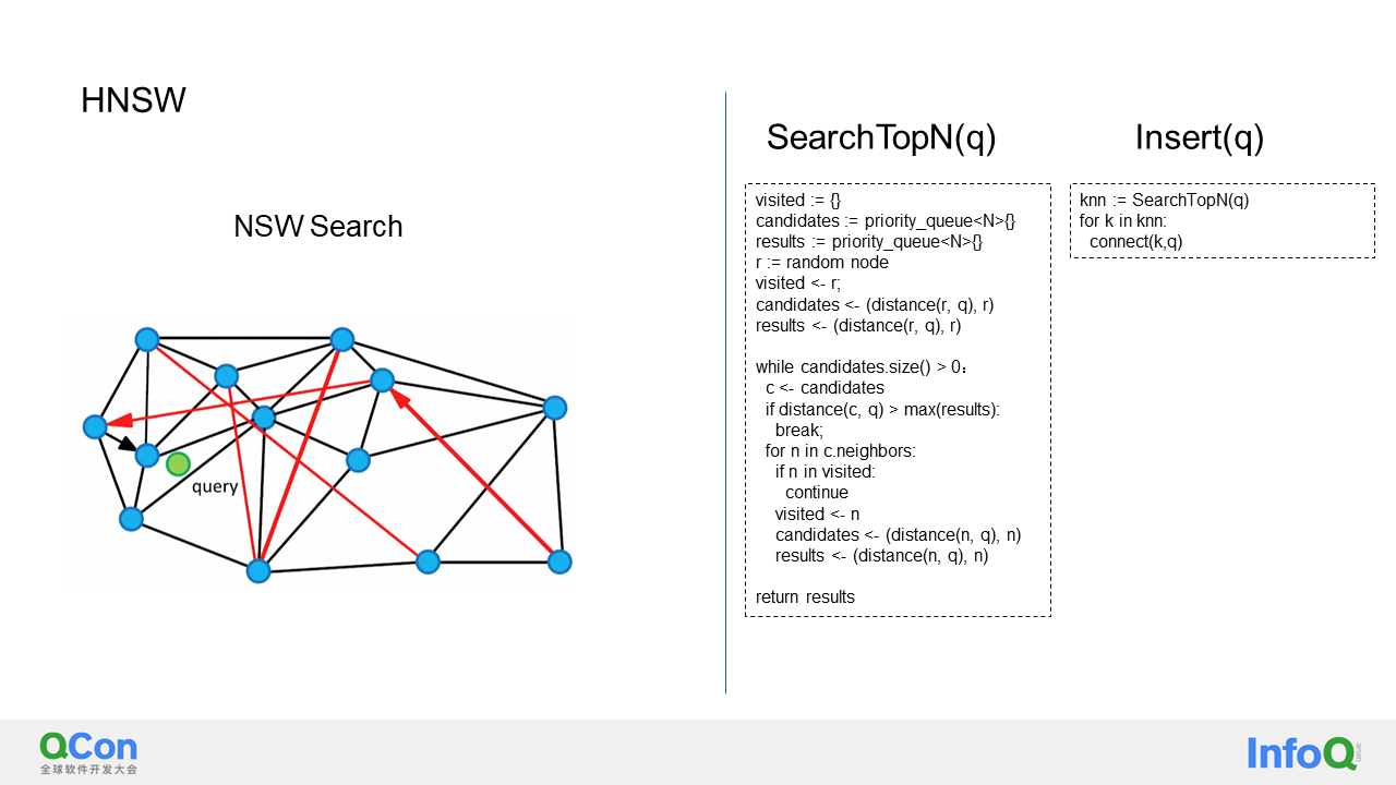
First of all, let's discuss the implementation of the search and insertion algorithms in NSW. I have provided a simple pseudo code for this purpose. The process begins with randomly selecting a node and adding it to a priority queue for bootstrapping.
Next, nodes are continuously retrieved from this priority queue. If the distance between the retrieved node and the target node is greater than the distances of all known answers, the search is stopped. Otherwise, all neighbors of the retrieved node are marked as visited and added to both the candidate's priority queue and the result set. This process continues until either all nodes are visited or clipped, or the specified upper limit on the number of visited nodes is reached. At this point, the algorithm returns the results, providing the approximate k nearest nodes to the target node. The insertion process is equally simple. During insertion, the algorithm runs the search algorithm to find the k nearest nodes to the newly inserted node and establishes connections with them.
HNSW is an extension of NSW that incorporates a hierarchical structure similar to a skip list. This structure allows for faster navigation to the node closest to the query node by utilizing the layers above. So, how does it achieve this? The search process is straightforward. When searching, I start from the top and search for the closest node at each layer until reaching the penultimate layer. At the penultimate layer, I can use that node as the starting point for the NSW query by employing the search method mentioned earlier.
Now, let's discuss how HNSW handles insertion. There are some differences during insertion because, in a data structure like a skip list, you must ensure that the node is inserted at the bottom layer (lc layer). To achieve this, a coin is tossed, and the result determines the highest layer at which the node will be inserted. During insertion, the algorithm follows the same procedure as before, searching for the closest node from the top layer to the layer being inserted. For each layer, the top n closest nodes are found, all the way from the layer to be inserted to the bottom layer. The main difference between this algorithm and the previous NSW algorithm is the addition of a function called SelectNeighbors.
This function performs a heuristic search to avoid the formation of detached islands, as shown in the diagram. The goal is to connect the two clusters in the HNSW diagram. The algorithm used in this case is as follows: If a candidate node is found, the distance from that node to the target node is calculated. If the distance is greater than the distance from a previously added node, the candidate node is temporarily skipped because it can also be connected through the previously added node. With a conventional algorithm, all nodes would be added to the candidate nodes. However, with the mentioned algorithm, some nodes are skipped. As a result, a node from another distant cluster has a chance to be added because it is closer to the green node than all other previously added nodes. This partially solves the problem of detached islands.
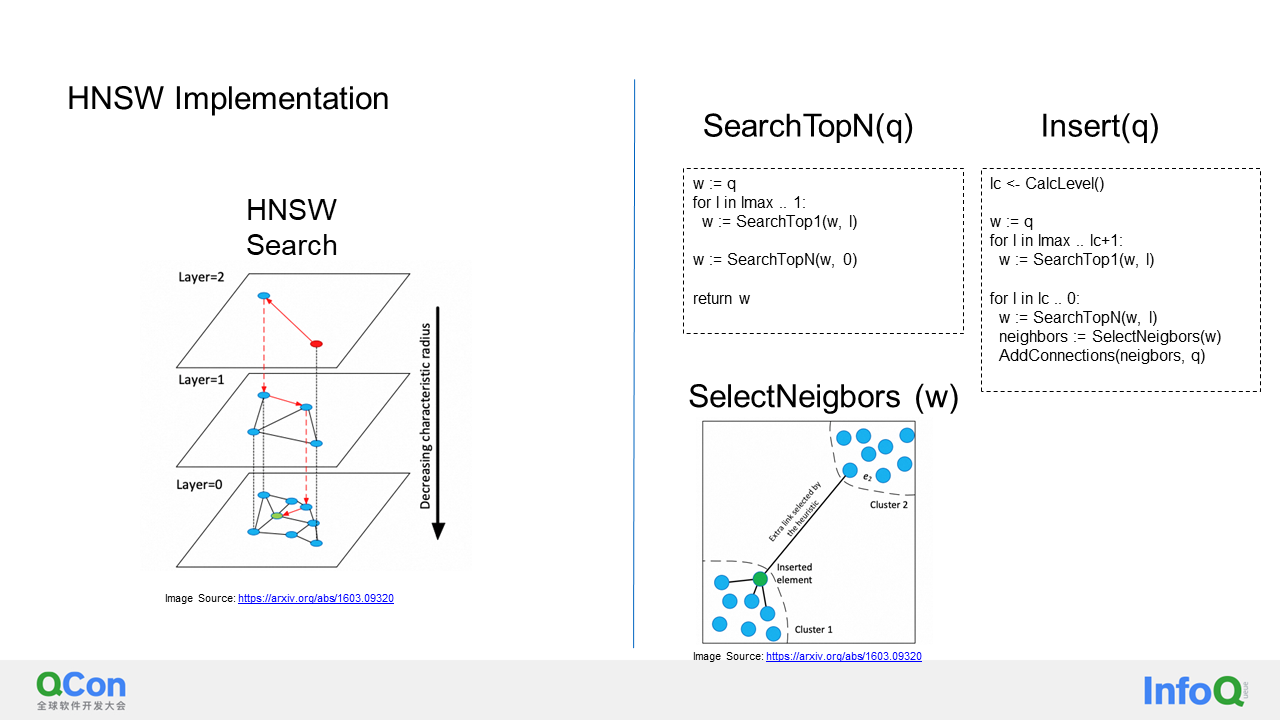
With the algorithm we just described, we also need a data structure and storage method to implement a vector database. As we know, AnalyticDB for PostgreSQL is based on PostgreSQL and natively supports its index interface. PostgreSQL provides a pluggable index structure. In this case, we adopt the paged segmentation memory method to store the points and edges of the HNSW separately. Each edge's page contains all edges with this point as the initial node at all layers, making it convenient for edge queries. Storing points and edges separately has several advantages:
First, it significantly reduces I/O. When searching, we may find a point but later determine that it doesn't meet the filtering conditions, so we discard it. If points and edges are stored together, reading the edges of the node becomes unnecessary and wasteful, but by storing them separately, we can reduce I/O.
Second, storing points and edges separately allows us to cache all pages of points in memory since the amount of data in points is much smaller than that in edges. This reduces the number of page openings.
Third, in order to handle concurrent scenarios, we need to lock all accesses to points and edges at the page level. Storing points and edges separately helps reduce conflicts and increase the concurrency and throughput of the entire system.
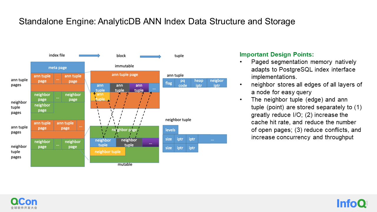
With the disk-based data structure and the algorithm just described, we have a functional vector database. However, when running it online, we discovered a performance issue, especially in scenarios with high-dimensional vectors, such as vectors with 1536 dimensions. In such cases, execution time is significantly increased. To address this, we have implemented an optimization called PQ encoding, which reduces the dimensionality of each vector.
PQ stands for Product Quantization. The concept is simple: the vector is divided into m blocks, and the K-means algorithm is applied to all vectors within each block. After that, each part of the vector is replaced with the K-means node that is closest to it. This reduces the dimension and accuracy of the entire vector. The calculations required are less CPU-intensive, resulting in faster overall processing speed. Additionally, the reduced length of the stored vector reduces the total storage size. However, it's important to note that the PQ codebook needs to be trained with offline data before encoding.
As a real-time data warehouse, AnalyticDB imports data in real-time, so there may be situations where no data is present when processing user data. To solve this "chicken or the egg" problem, we take an incremental approach. When there is no data, we perform calculations using the original vector. Once a threshold is reached, for example, when there are 100,000 pieces of data, we start a background process to calculate the codebook for these 100,000 vectors. After the codebook is calculated, the data that has been written is gradually backfilled. Meanwhile, newly written vector data can also be encoded using the newly trained codebook. This process is iterative. For example, when there are 100,000 pieces of data, the operation can be performed, and when there are 300,000 pieces of data, the operation can be performed again to improve accuracy when the data distribution changes. Even when there are 1 million pieces of data, this operation can be performed when the data distribution is relatively stable. The advantage of this approach is that accuracy keeps improving, and this training process is imperceptible to users in terms of queries and writes. After implementing this optimization, we have achieved a 5x increase in QPS and reduced the storage size to one-third of the original size.
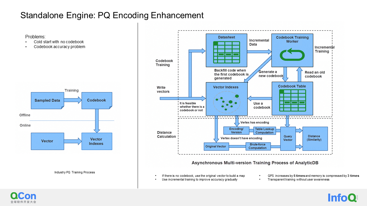
In this section, I will introduce how deletion is implemented in our vector database. Unlike many other vector databases on the market, our database supports deletion. One of the main reasons is that we are a real-time database, allowing users to delete their data whenever they want.
To minimize the noticeable delay caused by deletion, we use a two-step process. First, we mark the node to be deleted on the graph. Then, we return the user's deletion operation after the marking is done. This is because as users delete more data, the number of marked deletion points accumulate, and searching with all these points in the graph would be inefficient. Therefore, when the number of marked deletion points reaches a certain threshold, we start a background process to clean them up.
In the second, third, and fourth steps, we traverse the graph to find all the edges that point to the deleted node. These edges are then deleted. After deleting these edges, we can proceed to delete the node itself. However, deleting the node may cause issues in the graph. This is because when building the HNSW index, we ensure that the graph has connectivity. But when nodes and edges are deleted, the graph may become disconnected, affecting the recall rate. To address this, we move to the fourth step, which involves edge supplementation. Using an algorithm, we connect the deleted point with other edges around it to restore the graph's connectivity if the in-degree or out-degree of the point is not sufficient.
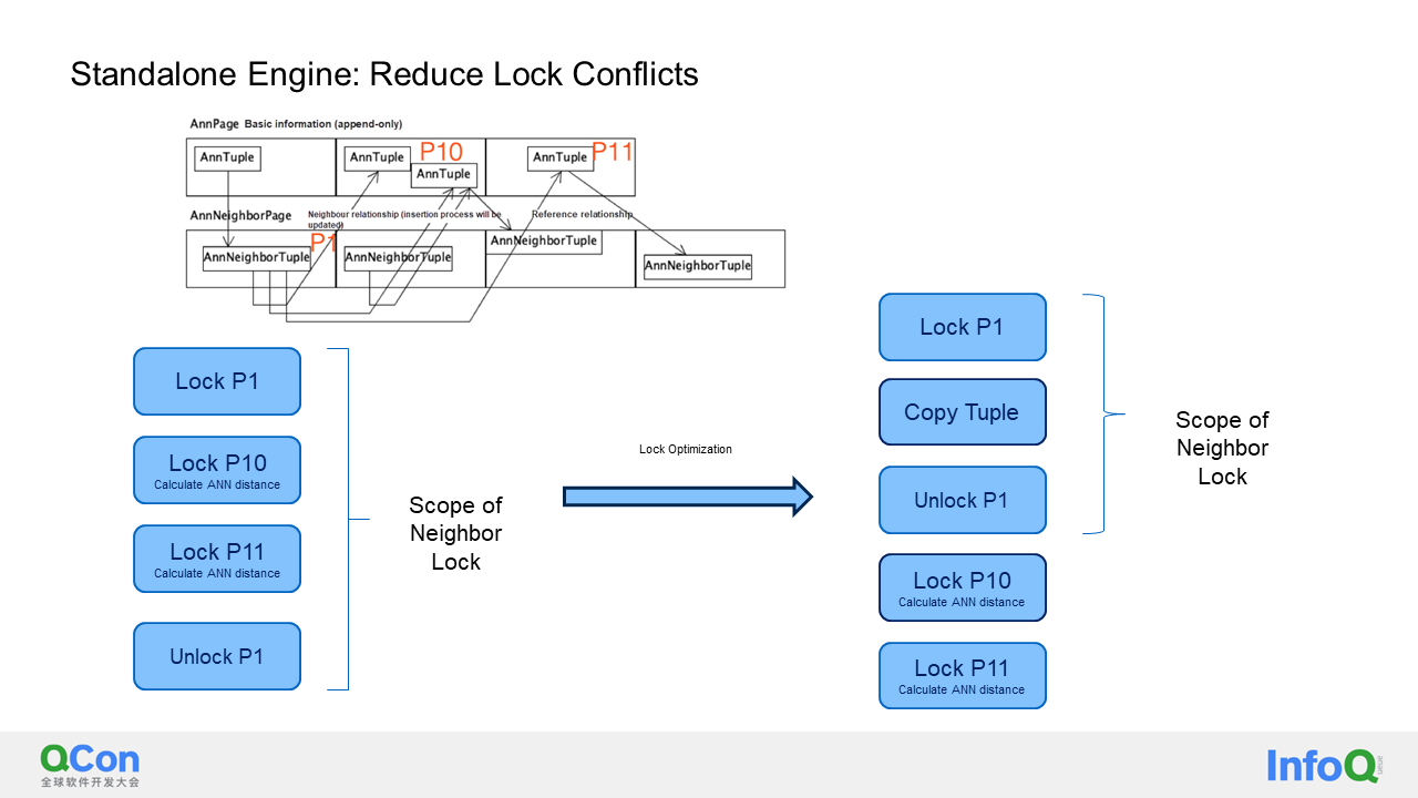
We have done a lot of optimization. In this section, I will focus on one of them: reducing lock conflicts. As you may know, when developing the HNSW algorithm, I used locks on these pages to ensure concurrency correctness. If implemented directly, you would lock page 1. Then, you would need to find its adjacent edges and lock page 10 and page 11. Only after the calculation is complete can you unlock page 1. Although I have only shown two points here, in reality, there may be a large number of points to be calculated on this page. Moreover, there might be many pages to be accessed as well. This locking method reduces the overall system throughput because other concurrent queries may have to wait for locks.
To address this problem, we have a simple solution. After locking page 1, we make a copy of the tuple to be calculated. Then, we unlock page 1, and the distance of the vector can be calculated using the unlocked tuple. Additionally, we perform an optimistic test to ensure that write-write conflicts do not result in data loss.
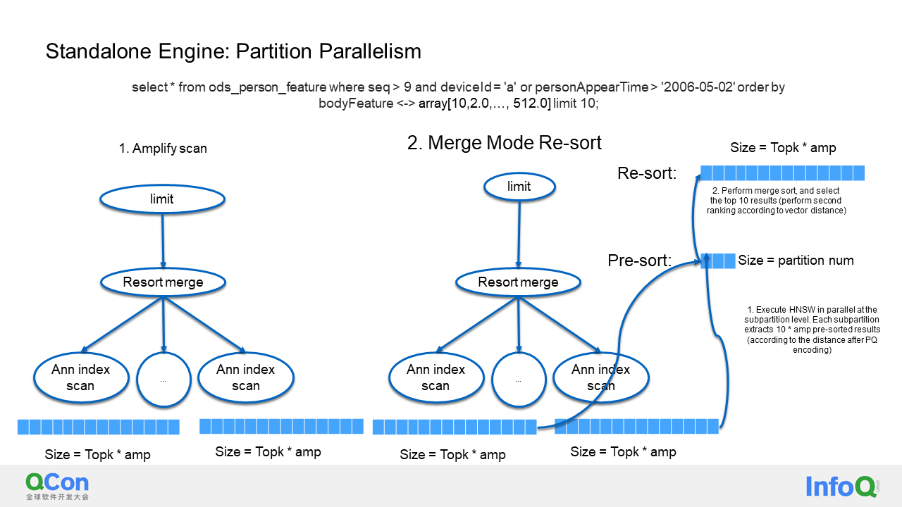
In this section, I will discuss the concurrent execution of partitions. As we know, our database can be divided into partitions, such as time partitions. For each partition, there is an HNSW index, and I will multiply the top k by an amplification factor for each index. This amplification factor exists to compensate for the reduced recall rate after PQ encoding, even if it is not a partitioned table. Essentially, each partition is executed concurrently by threads. After execution, each partition selects the top k and multiplies the numbers by the amplification factor. Then, a merge sort is implemented as a second-ranking process, using the real vector distance for all operations. This step accelerates the efficiency of ANN vector search for partitioned tables.
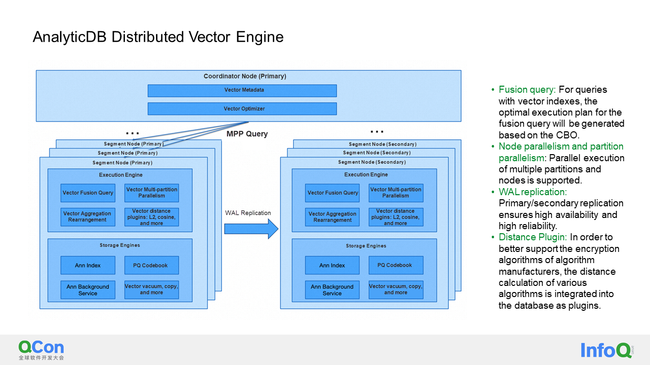
In the previous sections, I discussed how to implement a vector engine and optimize it on a standalone machine. AnalyticDB, being a distributed system, naturally incorporates its distributed capability into the entire vector database. AnalyticDB follows an MPP architecture, where data is sharded by hash, determining which node each piece of data goes to based on the hashing of the distribution key.
There are two levels of concurrency granularity in this architecture. The first is node-level concurrency, and the second is partition-level concurrency within each node. Therefore, the concurrency is multiplied by the partition level. To ensure high reliability and availability, each node has a primary shard and a secondary shard. The primary and secondary shards are synchronized through write-ahead logging, resulting in two copies of the data for high reliability. In the event of a primary shard failure, a detection system automatically switches to the secondary shard within ten seconds, ensuring high availability. In addition to the distance calculation methods mentioned earlier, we also support distance algorithms developed by algorithm manufacturers, which can be integrated into our vector database via distance plugins.
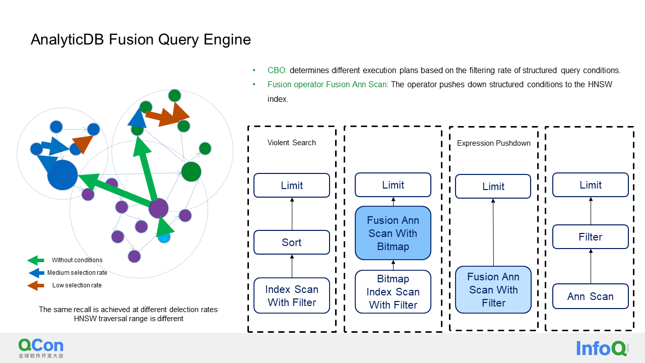
In this section, I will provide a detailed explanation of the fusion query. The fusion query aims to solve the problem of querying both structured and unstructured data in a data system simultaneously. This means that an SQL statement can check vectors and filter structured data at the same time. The main goal of the fusion query is to execute this SQL statement as efficiently as possible.
To achieve this, we use CBO (Cost-Based Optimizer) to determine which of the following four paths to choose.
The HNSW (Hierarchical Navigable Small World) scan operator, in the second step, has the capability to push the filter or bitmap down to it for execution. This means that if I have a query condition that looks up the top k of a vector, and I also have another structured field with a filter condition such as greater than 3 or less than 5, I will first use the optimizer to determine the filtering rate of this structured data. If the filtering rate is low, which means that only a few structured data will be filtered out, I have a simple execution method to solve the problem. I will first retrieve all the filtered data and then perform a brute-force vector scan on these data. This method is the most efficient one. However, if the optimizer indicates that the filtering rate is not low, I will first execute a bitmap index scan to filter the structured data and then push the bitmap into my vector index for execution.
In the third scenario, if the filtering rate is higher, the bitmap may become very large. In this case, the whole calculation expression will be pushed to the HNSW scan operator.
In the fourth scenario, the entire filter has little to no effect. In this case, HNSW must be calculated first and then filtered because the filter cannot filter out many pieces of data. You may wonder why we don't always carry out the fourth process directly. The disadvantage of doing so is that HNSW may calculate the top k pieces, but those pieces of data may not meet the filter conditions. As a result, only a small number of pieces of data will be filtered out, which fails to meet the user's query requirements.
In this section, I will present some real-life use cases. The first case involves a pure vector search process in an image-based search system. To ensure data privacy, I will use a photo of my dog (named Snoopy) as an example. However, you can imagine that the same process can be applied to license plate or facial recognition.
The scenario here is that I have a large number of IoT devices, and one of them keeps taking pictures. These pictures are continuously uploaded to the vector database in real-time. Now, suppose my dog goes missing, and I want to know its whereabouts. I can input a photo of my dog into the vector database for searching, and similar photos will be quickly found within milliseconds. It is important to note that our vector database supports real-time writing with a capacity of tens of thousands of QPS (Queries Per Second), and each query can return results within milliseconds.
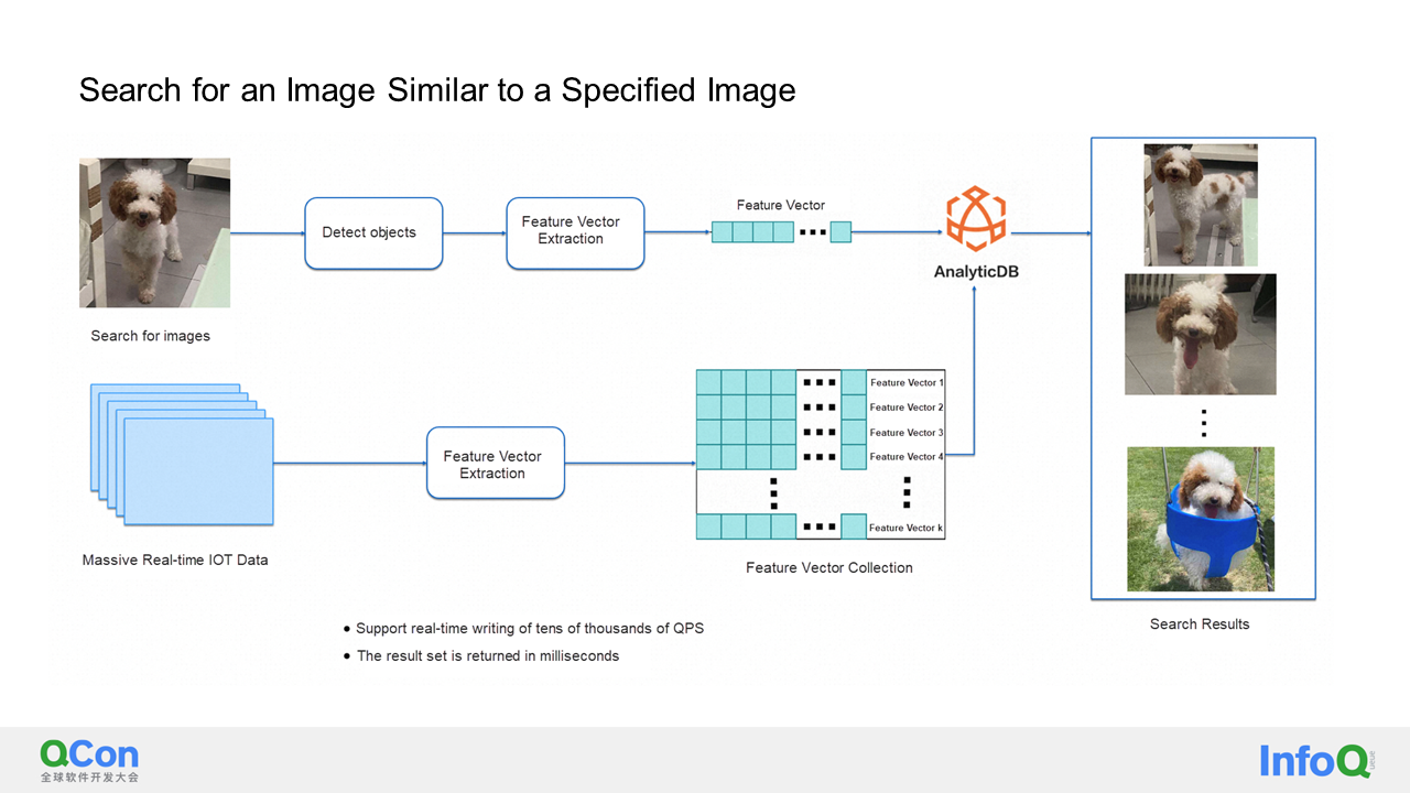
In the AIGC scenario, especially in the past six months, we have discovered that users require more than just the capabilities of a vector database. They also need two additional functionalities.
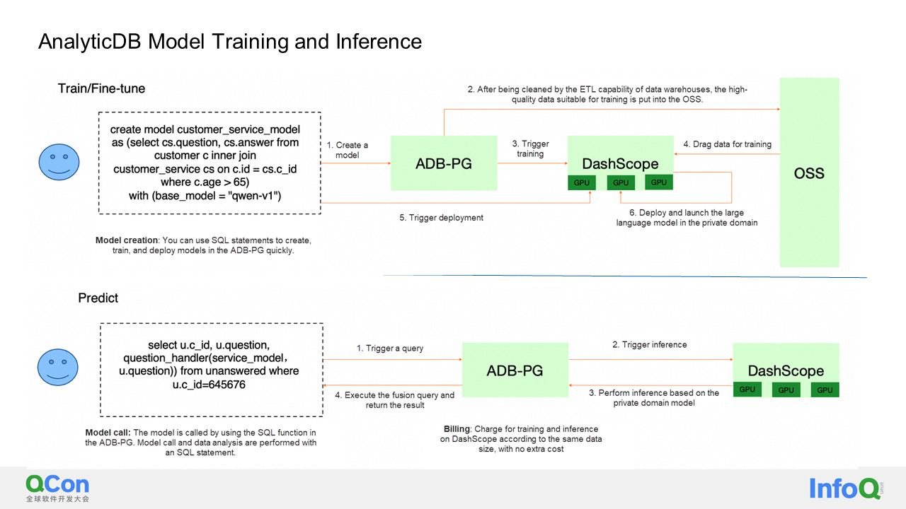
So what are these two additional functionalities? I have already explained the first one. It involves the ability to understand documents that are being inputted. What does this mean? Let's say we have a document with different levels of titles and a body. If we randomly segment the document, the body may be incorrectly associated with the wrong title due to the segmentation method used. This can negatively affect search results. With the ability to understand documents, we can re-attach the correct title to the segmented text, making it easier to comprehend.
Additionally, customers also require a reliable segmentation algorithm, especially for Chinese text. We have also developed the capability to generate embeddings. All of these functionalities have been integrated into an HTTP service that we have deployed within our vector database. The second part involves our ongoing efforts to combine these capabilities with a large language model. We aim to fine-tune the model within the vector database and implement model-based inference.
In conclusion, our approach is to store users' structured data, JSON text, and vector data in a comprehensive data system that addresses all their data analysis needs.
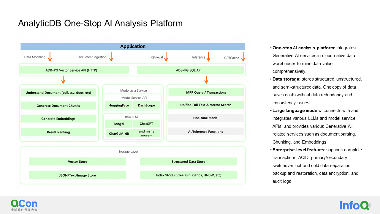
Finally, I would like to discuss the work we are currently undertaking. The first project involves the separation of compute and storage for vectors. As I mentioned earlier, we store vectors in local storage. However, for the HNSW index, we need to frequently perform update and delete operations, which are not compatible with cloud-native DFS systems that are append-only or write-once-never-modify.
Initially, we implemented solution 1 as shown in the figure. This was because in the data writing process, the data was first written into the Delta table using row-oriented storage. Then, when the Delta table reached a certain size, we would transfer it to DFS and store it in the form of column-oriented storage, which improved scanning speed. Therefore, each time a fragment was transferred, we also built a small HNSW index because the fragment was immutable. When querying, we actually queried these indexes separately and then merged the results. If there was a delete operation, we stored it in memory first, and when the number of delete operations reached a certain threshold, we performed compaction with the following fragments and then rewrote the fragment. However, we found that Scheme 1 had a problem. We couldn't find a suitable balance. For example, if we wanted a high recall rate, we had to set the recall rate of each HNSW index very high. However, this was inconsistent with the compute-storage architecture I described earlier. In the compute-storage architecture, there was one shard and one HNSW index, but in this case, there was one fragment and one HNSW index. Therefore, after performing a vector search, we needed to merge these very small results, which incurred high costs. On the other hand, if we reduced the value of k (the number of results to be retrieved), we found that the recall rate was not effective. Therefore, we ultimately abandoned this scheme and adopted Scheme 2.
Scheme 2 is very simple. We shouldn't limit ourselves to the idea that compute-storage separation can only be achieved through pure immutable shared storage. Instead, we built a multi-tenant storage pool. This storage pool stores pages of HNSW points and edges and is shared by multiple instances. Resource planning for the storage pool is done at the region level, and it does not require frequent scaling in and scaling out. When writing, data is first written into the log keeper service. Then, the log keeper sends these logs to the page server. When reading, the page server applies the logs as needed to create a new page based on the original page. No data is stored locally on the compute node. This approach guarantees both performance and the previously adjusted recall rate, and has minimal impact on the original code.
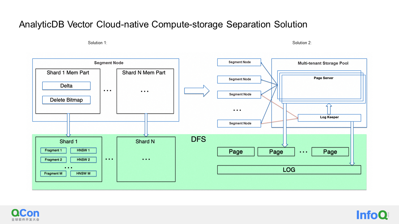
Finally, I will explain how our vector database is integrated with DashScope. If you want to fine-tune a model, the data must be cleaned and of high quality. We aim to clean the data in the AnalyticDB cloud-native data warehouse and also train models in AnalyticDB. When writing a SQL statement, the ETL capabilities will first clean the data and write it to OSS. Then, during model training, we call the DashScope service to import this data and fine-tune it based on a specific model, such as Qwen v1. After fine-tuning, we can trigger the launch and deployment of the entire model, integrating the fine-tuning, launch, and deployment processes into the SQL statement. Additionally, we can use AnalyticDB for inference. Users can write a UDF (User-Defined Function) and call the pre-trained and deployed model to perform inference. For example, if there is an after-sales Q&A service, we can fine-tune the model using high-quality after-sales Q&A data that has been manually answered. After fine-tuning, when new questions come in, we only need to call this model to automatically generate replies, improving the user experience.
That's all for my sharing. Thank you!
Yiwei Yao is the head of AnalyticDB for PostgreSQL, an Alibaba Cloud cloud-native data warehouse, and a senior technical expert of Alibaba. He is committed to building ultra-large-scale serverless cloud-native data warehouses. He graduated from Stanford University in 2011 with a master's degree in computer science. After joining Alibaba in 2020, he has been committed to overcoming technical difficulties, such as online and offline integration, lake house, and serverless technology, achieving real-time online data services with second-level elasticity, mixed hot and cold data storage, extremely compressive and cost-effective proprietary data format, intelligent optimizer, resource isolation in mixed load and multi-tenant scenarios, and exclusive vector capabilities in AIGC scenarios.
One-Stop Data Management & Data Serving Platform | Alibaba Cloud Developer Summit 2023 Recap
[Infographic] Highlights | Database New Feature in November 2023
ApsaraDB - June 16, 2023
Alibaba Cloud Indonesia - July 5, 2023
ApsaraDB - March 20, 2024
Alibaba Cloud Indonesia - July 5, 2023
Farah Abdou - December 5, 2025
ApsaraDB - February 13, 2021
 AnalyticDB for MySQL
AnalyticDB for MySQL is a real-time data warehousing service that can process petabytes of data with high concurrency and low latency.
Learn More AnalyticDB for PostgreSQL
An online MPP warehousing service based on the Greenplum Database open source program
Learn More Database for FinTech Solution
Leverage cloud-native database solutions dedicated for FinTech.
Learn More PolarDB for MySQL
Alibaba Cloud PolarDB for MySQL is a cloud-native relational database service 100% compatible with MySQL.
Learn MoreMore Posts by ApsaraDB