By Zhang Shiliang, Senior Algorithm Engineer
At the recently held Computing Conference Wuhan Summit, an AI cashier installed with the Deep Feedforward Sequential Memory Network (DFSMN), a speech recognition model, competed with human cashiers. It accurately recognized customers' speech in a noisy environment and ordered 34 cups of coffee within 49 seconds. Ticket vending machines (TVMs) with the speech recognition technology have also been deployed at the Shanghai Metro.
Xie Lei, a well-known speech recognition expert and professor of Northwestern Polytechnical University, said, "Alibaba Cloud's open source DFSMN model breaks through the barrier for improving speech recognition accuracy. It is one of the most representative achievements of deep learning in the speech recognition field in recent years, and greatly impacts both the global academic industry and AI technology applications."
Alibaba Cloud makes its speech recognition model DFSMN open source on the GitHub platform
Speech recognition technology has always been an important part of human-machine interaction technology. With the speech recognition technology, machines can recognize speech as human beings, allowing them to think, understand, and provide feedback.
With the application of deep learning technology in recent years, the deep neural network (DNN)-based speech recognition system has been greatly improved in terms of performance and is progressively being used in practice. Speech recognition-based speech input, speech transcription, speech retrieval, and speech translation technologies have also been widely applied.
Currently, the mainstream speech recognition systems commonly use the acoustic model based on the deep neural network-hidden Markov model (DNN-HMM), whose structure is shown in Figure 1. The input of the acoustic model is the spectral features extracted from traditional speech waveforms after they are processed by windowing and framing. Examples of the extracted features are perceptual linear prediction (PLP), mel-frequency cepstral coefficients (MFCC), and filter banks (FBKs). The output of the acoustic model is the acoustic modeling units of different granularities, such as mono-phone, mono-phonestate, and binding tri-phonestate. Different neural network structures can be used between the input and output. The input acoustic features are mapped to obtain the posterior probabilities of different output modeling units. Then, the final recognition results are obtained by decoding the HMM.
The earliest used neural network structure is the feedforward fully-connected neural network (FNN). The FNN implements one-to-one mapping of fixed input to fixed output. However, the FNN cannot effectively use the intrinsic long-range dependence (LRD) information of speech signals. An improved solution is to use a recurrent neural network (RNN) based on the long-short term memory (LSTM). Through the recurrent feedback connection at the hidden layer, the LSTM-RNN can store historical information on the nodes at the hidden layer to effectively use the LRD of speech signals.
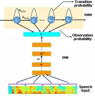
Figure 1: Block diagram of the speech recognition system based on the DNN-HMM
By using a bidirectional RNN, historical and future information of speech signals can be effectively used, facilitating the acoustic modeling of speech. The RNN-based speech acoustic model provides better performance than the FNN-based speech acoustic model. However, the RNN-based speech acoustic model is more complex and contains more parameters, requiring more computing resources for model training and testing.
In addition, the bidirectional RNN-based speech acoustic model may cause a high latency, making it unsuitable for real-time speech recognition tasks. To address this, some improved models are provided, such as the latency controlled LSTM (LCBLSTM) [1-2] and the feedforward sequential memory network (FSMN) [3-5]. Last year, Alibaba Cloud launched the first LCBLSTM-based acoustic model for speech recognition in the industry. With Alibaba Cloud's MaxCompute, the acoustic modeling was carried out by using the multi-machine multi-GPU, 16-bit quantization, and other training and optimization methods. The LCBLSTM-based acoustic model achieved 17% to 24% word error rate (WER) reduction compared with the FNN model.
FSMN is a recently proposed network structure. Learnable memory blocks are added at the hidden layer of the FNN to effectively model the LRD of speech. Compared with LCBLSTM, FSMN controls latency more conveniently, provides better performance, and requires less computing resources. However, it is difficult for the standard FSMN to train very deep structures, and the training effect is poor because of the vanishing gradient problem. Given that deep structured models are proven to have more modeling capabilities in many fields, we have proposed an improved FSMN model, namely, deep FSMN (DFSMN). Furthermore, we have developed an efficient, real-time acoustic model for speech recognition based on low frame rate (LFR) technology. Compared with the LCBLSTM launched last year, this acoustic model ensures an over 20% relative performance improvement and two to three times acceleration in training and decoding. It significantly reduces computing resources required in practice.
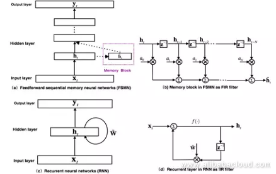
Figure 2: FSMN model structure and comparison with the RNN
Figure 2 (a) shows the structure of the FSMN [3], which is essentially an FNN. Memory blocks are added at the hidden layer to model the context, thus modeling the LRD of time series signals. The memory block uses the tapped-delay line structure shown in Figure 2 (b) to encode the hidden layer output of the current moment and the previous N moments by a group of coefficients to obtain a fixed expression. The proposed FSMN is inspired by the filter design theory in digital signal processing: Any infinite impulse response (IIR) filter can be approximated by using a high-order finite impulse response (FIR) filter. From the perspective of the filter, the recurrent layer of the RNN model shown in Figure 2 (c) can be regarded as the first-order IIR filter shown in Figure 2 (d). The memory block that the FSMN uses, as shown in Figure 2 (b), can be regarded as a high-order FIR filter. Similar to the RNN, the FSMN can also effectively model the LRD of signals. Because the FIR filter is more stable than the IIR filter, the FSMN is simpler and more stable than the RNN in training.
Based on the encoding coefficients of the memory block, FSMNs can be classified into scalar FSMN (sFSMN) and vectorized FSMN (vFSMN). The sFSMN and vFSMN use scalars and vectors, respectively, as the encoding coefficients of the memory block. The sFSMN and vFSMN memory blocks are expressed by using the following formulas:
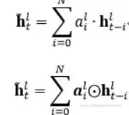
The preceding FSMN only considers the impact of historical information on the current moment and is called a one-way FSMN. Considering the impact of both historical information and future information on the current moment, we can extend the one-way FSMN to the two-way FSMN. The memory blocks of the two-way sFSMN and vFSMN are encoded by using the following formulas:
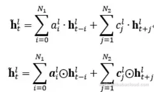
where N1 and N2 indicate the look-back order and the look-ahead order, respectively. We can enhance the ability of the FSMN to model the LRD by increasing the order or by adding memory blocks at multiple hidden layers.
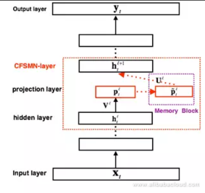
Figure 3: Block diagram of the cFSMN structure
Compared with the FNN, the FSMN DFSMN needs to use the output of the memory block as an additional input to the next hidden layer, which introduces additional model parameters. The more nodes the hidden layer contains, the more parameters are introduced. Based on the idea of low-rank matrix factorization, the research [4] proposes an improved FSMN structure, namely, compact FSMN (cFSMN). It contains memory blocks at the I-th hidden layer.
For the cFSMN, a low-dimensional linear projection layer is added after the hidden layer of the network. Memory blocks are added to these linear projection layers. The encoding formula of the memory block in the cFSMN is also modified. The output at the current moment is explicitly added to the expression of the memory block, which is used as the input for the next layer. This effectively reduces the number of parameters of the model and speeds up the network training. The formulas for expressing the memory blocks of the one-way and two-way cFSMNs are as follows:
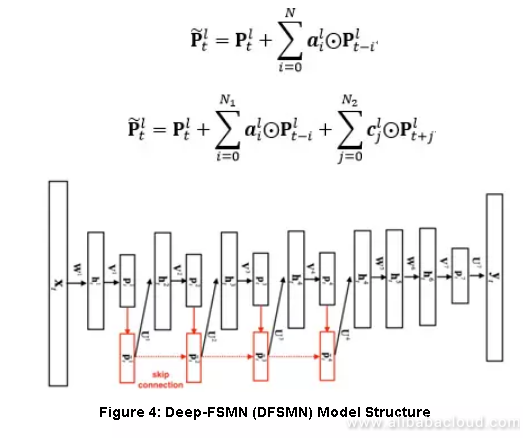
Figure 4 is the block diagram of the DFSMN structure. The leftmost box indicates the input layer. The rightmost box indicates the output layer. We have added skip connections between the memory blocks (represented by red boxes) of the cFSMN. In this way, the output of a lower-layer memory block is directly added to an upper-layer memory block. In the training process, the gradient of the upper-layer memory block is directly assigned to the lower-layer memory block. This helps overcome the vanishing gradient problem caused by the depth of the network and ensure stable training of deep networks. We have also modified the expression of the memory block. By referring to the idea of dilation convolution [6], we import some stride factors into the memory block. The calculation formula is as follows:

where,
 indicates the output of the l-1 layer memory block at the t-th moment. S1 and S2 indicate the encoding stride factors at the historical and future moments, respectively. For example, if the value of S1 is 2, a value is taken every other moment as the input to encode the historical information. This allows a longer history to be viewed in the same order and helps model the LRD more effectively.
For the real-time speech recognition system, we can control the latency of a model by flexibly setting the future order. In extreme cases, when the future order of each memory block is set to 0, an acoustic model without latency can be provided. For some tasks, we can tolerate a certain amount of latency, and therefore we can set a smaller future order.
The advantage of the DFSMN over the cFSMN is that skip connections can be used to train very deep networks. Each hidden layer in the previous cFSMN has been split into two layers with low-rank matrix factorization. For a network with four cFSMN layers and two DNN layers, the total number of layers is 13. If more cFSMN layers are added, the number of layers increases and the vanishing gradient problem occurs, resulting in unstable training. The proposed DFSMN uses skip connections to avoid the vanishing gradient problem of deep networks, improving the training stability for deep networks. Note that skip connections can be added not only between adjacent layers but also between non-adjacent layers. A skip connection can be either a linear or nonlinear transformation. In experiments, a DFSMN network with dozens of layers has been trained, with significant performance improvement compared with the cFSMN.
From the original FSMN to the cFSMN, we can not only effectively reduce model parameters, but also achieve better performance [4]. The proposed DFSMN based on the cFSMN can further significantly improve the performance of the model. The following table compares the performance of different acoustic models based on the BLSTM, cFSMN, and DFSMN in a 2000-hour English recognition task.

The preceding table indicates that the WER of the DFSMN model is reduced by 14% compared with that of the BLSTM acoustic model in the 2000-hour task. The DFSMN significantly improves the performance of the acoustic model.
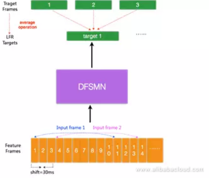
Figure 5: Block diagram of the LFR-DFSMN-based acoustic model
The input of the current acoustic model is acoustic features extracted from each frame of the speech signal. The duration of each speech frame is generally 10 ms. An output target is set for each input speech frame. Recently, research has proposed an LFR [7] modeling scheme: The speech frames at adjacent moments are bound as input to predict the average value of the output targets of these speech frames. In experiments, three or more frames can be collaged without compromising the performance of the model. Thus, the input and output can be reduced to one-third or more, greatly improving the acoustic score calculation and decoding efficiency when the speech recognition system works. Based on the LFR and the preceding DFSMN, we set up the LFR-DFSMN-based acoustic model for speech recognition, as shown in Figure 5. After multiple experiments, the DFSMN with ten cFSMN layers and two DNN layers was determined as the acoustic model that should be used. The input and output are in LFR mode, reducing the frame rate to one-third. The following table compares the performance of the LFR-DFSMN-based acoustic model and the best performance of the LCBLSTM acoustic model launched last year.

By combining LFR technology, we can achieve three times acceleration in recognition. As described in the preceding table, the LFR-DFSMN model achieves a 20% CER reduction compared with the LFR-LCBLSTM model in practical industry applications. It presents better modeling features for large-scale data.
The actual speech recognition service usually needs to process complex speech data. The acoustic model for speech recognition must cover as many scenarios as possible, including various dialogs, channels, noises, and even accents. This means that massive data is involved. How to apply massive data to quickly train an acoustic model and bring the service online directly affects the business response speed.
We use Alibaba Cloud's MaxCompute platform and multi-machine multi-GPU parallel training tool for training. The following table describes the training speeds of the LFR-DFSMN and LFR-LCBLSTM acoustic models when 8 machines, 16 GPUs, and 5,000 hours of training data are provided.

Compared with the baseline LCBLSTM model, the DFSMN can achieve three times the training speed in terms of each epoch. When the LFR-DFSMN is trained in a 20,000-hour task, the model convergence only takes three to four epochs. When 16 GPUs are provided, a 20,000-hour training task for the LFR-DFSMN acoustic model can be completed in about two days.
To design a more practical speech recognition system, we must consider improving the system recognition performance whenever possible and ensuring the system timeliness to provide a better user experience. In addition, the service cost must be considered in practice. The power consumption of the speech recognition system must meet certain requirements. The traditional FNN system requires frame collage. The decoding latency usually consumes 5 to 10 frames, that is, 50 to 100 ms. The LCBLSTM system launched last year solves the whole sentence latency of the BLSTM and controls the latency to about 20 frames, that is, 200 ms. For some online tasks with higher requirements on the latency, the LCBLSTM can control the latency to 100 ms at the slight expense of recognition performance (0.2% to 0.3% absolute value), which fully meets the needs of various tasks. The LCBLSTM can achieve a relative performance improvement of more than 20% compared with the best FNN. However, the recognition speed of the LCBLSTM is slower because of high power consumption in the same CPU conditions. This is largely caused by the complexity of the model.
With LFR technology, the latest LFR-DFSMN can accelerate the recognition speed over three times. The DFSMN can achieve a model complexity reduction of about three times that of the LCBLSTM. The following table describes the recognition time required for different models collected in a test set. A shorter time indicates a lower computation power requirement.
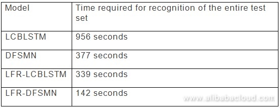
The decoding latency of the LFR-DFSMN can be reduced by reducing the future order of the memory block filter. Different configurations have been verified in experiments. The results show that only 3% of performance is lost when the latency of the LFR-DFSMN is controlled to 5 to 10 frames.
In addition, compared with the complex LFR-LCBLSTM model, the LFR-DFSMN model is more simplified. Although the LFR-DFSMN contains ten DFSMN layers, the overall model size is only half that of the LFR-LCBLSTM model, with the model size compressed by 50%.
Using DataX-On-Hadoop to Migrate Data from Hadoop to MaxCompute

137 posts | 21 followers
FollowPM - C2C_Yuan - April 16, 2024
Alibaba Clouder - October 11, 2019
Alibaba Cloud Product Launch - December 12, 2018
Alibaba Clouder - March 31, 2021
Alibaba Clouder - July 12, 2018
Alibaba Cloud Community - January 7, 2022

137 posts | 21 followers
Follow Intelligent Speech Interaction
Intelligent Speech Interaction is developed based on state-of-the-art technologies such as speech recognition, speech synthesis, and natural language understanding.
Learn More Big Data Consulting for Data Technology Solution
Alibaba Cloud provides big data consulting services to help enterprises leverage advanced data technology.
Learn More MaxCompute
Conduct large-scale data warehousing with MaxCompute
Learn More Big Data Consulting Services for Retail Solution
Alibaba Cloud experts provide retailers with a lightweight and customized big data consulting service to help you assess your big data maturity and plan your big data journey.
Learn MoreMore Posts by Alibaba Cloud MaxCompute