About Database Kernel | PolarDB Optimizer Query Transformation - Join Condition Pushdown

By Chen Liang (Yaoling)

Introduction

The database query optimizer is like the brain of the entire system. The efficiency of executing an SQL statement can vary significantly based on different optimization decisions. Therefore, the optimizer is one of the core components and competitive advantages of a database system. Alibaba Cloud PolarDB for MySQL is a cloud-native database that can handles various user scenarios and loads, helping enterprises go online and increase their data value. To enhance its capabilities, we have focused on improving the query transformation functionality of PolarDB for MySQL.

This article series will focus on the query transformation capability of PolarDB for MySQL and introduce some of our accumulated work in this direction.

This is the third article in the PolarDB Optimizer Query Transformation series. The first two articles explain the following topics:

1. Join elimination
2. Window functions

Preface

In the query optimization characteristics of the database, equivalent transformations based on relational algebra have always been a challenging but highly rewarding area, commonly referred to as query transformation. Many transformations can be heuristically applied (known as brainless transformations) by strictly verifying that there is no performance rollback. This often results in significant performance improvements, usually by one to two orders of magnitude. Join elimination is an example of heuristic application.

By using the window function of MySQL 8.0 to expand correlated subqueries, performance gains without rollback can be achieved when specific preconditions are met. For more information, see Database Kernel Things | PolarDB Optimizer Query Transformation - Window Functions. The window function-based decorrelation has greatly improved the performance of PolarDB TPC-H Q2 and Q17.

However, there is a better solution available here: http://oysteing.blogspot.com/2021/05/transformations-of-correlated-scalar.html

In his previous analysis of Q17, Oystein, a senior optimizer architect of the SQL team, mentioned a transformation scheme based on a lateral derived table. This scheme offers more stable performance and a higher acceleration ratio.

SELECT SUM(l_extendedprice) / 7.0 AS avg_yearly
FROM lineitem
  JOIN part ON p_partkey = l_partkey
WHERE p_brand = 'Brand#34'
  AND p_container = 'MED BOX'
  AND l_quantity < (
    SELECT 0.2 * AVG(l_quantity)
    FROM lineitem
    WHERE l_partkey = p_partkey
);

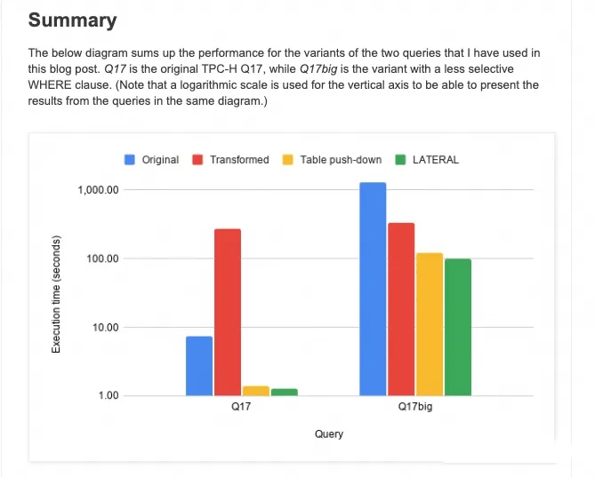
In the above figure, Q17big adjusts the selection rate of the part table in the outer query, while Table pushdown is a solution similar to a window function. We can observe that the performance of LATERAL is optimal in both cases. So, what exactly is the transformation involving LATERAL?

SELECT SUM(l_extendedprice) / 7.0 AS avg_yearly
FROM lineitem
  JOIN part ON p_partkey = l_partkey
  JOIN LATERAL((
    SELECT 0.2 * AVG(l_quantity)
    FROM lineitem
    WHERE l_partkey = p_partkey
  ))  AS ldt (avg_qty)
WHERE p_brand = 'Brand#34'
  AND p_container = 'MED BOX'
  AND l_quantity < avg_qty;

Here, a JOIN LATERAL and a derived table ldt with correlation are generated. The corresponding execution plan is as follows:

It may be difficult to understand how to jump from the original Q17 to such a plan. Let's look at it step by step:

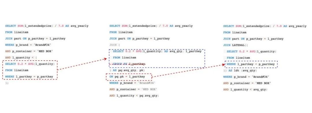
● Based on the original correlated subquery, the first step is to transform it into a derived table with a group by condition: pq(avg_qty, pk). Then, join this derived table with the part table or lineitem table in the outer query. Since the correlated condition is used as the group by column, the derived table only includes the data of the corresponding group for each row in the outer query, ensuring consistency with the original correlated subquery results. However, there is a problem:

The derived table pq requires a full table scan of the lineitem table, and then completing the aggregation calculation and materializing it at one time

Considering that the lineitem table has the largest data volume in TPC-H, this decorrelation approach does not guarantee better performance. This transformation has been implemented in PolarDB but is not enabled by default.

The second step is to further push down the Join condition pq.pk=l_partkey to the derived table pq. It becomes the form of a lateral derived table, which is equivalent to pushing down the Join condition based on the left-side transformation. This brings about three changes:

The inner layer adds a filter condition l_partkey=p_partkey. Indexes may be utilized to filter a large amount of data in the lineitem table.
The pushed-down condition covers all fields in the group by clause. Each time a row of data is generated in the outer layer, the inner layer always calculates the data for a specific group. The group by clause is no longer required and can be eliminated.
An ldt table needs to be materialized repeatedly. However, if the part table on which it depends has a relatively small amount of data, repeated materialization is cheaper than one full materialization.

Based on the above three factors, this transformation brings significant performance improvement and has a greater impact than window functions. However, it should be noted that there are many uncertainties involved. In other words, this is not a heuristic brainless transformation and needs to be determined based on cost.

Due to the high complexity of its implementation, it was not initially included in the short-term research and development plan. However, later on, online customers encountered the following practical problems:

SELECT *
FROM (
  SELECT *
  FROM db_order.tb_order
  WHERE create_date >= DATE_SUB(CAST('xxxx' AS datetime), INTERVAL 5 MINUTE)
    AND product_type IN (?, ?)
) o
  LEFT JOIN (
        ...
  ) od
  ON o.order_id = od.order_id
  LEFT JOIN (
    SELECT t.*, row_number() OVER (PARTITION BY detail_id ORDER BY update_date DESC) AS rn
    FROM db_order.tb_order_sku t
    WHERE update_date >= DATE_SUB('xxxx', INTERVAL 50 MINUTE)
      AND coalesce(product_type, 'xx') <> '?'
  ) os
  ON od.id = os.detail_id
...

The query has been simplified and blurred a lot, but the overall problem is: for the derived table os, because the inner table tb_order_sku has a large amount of data and does not have a suitable index, it needs to do a lot of aggregation calculation and materialize a large amount of data. Through repeated optimization, the manual rewriting is as follows:

SELECT *
FROM (
...
) o
LEFT JOIN (
...
) od
ON o.order_id = od.order_id
LEFT JOIN LATERAL((
    SELECT t.*, row_number() OVER (PARTITION BY detail_id ORDER BY update_date DESC) AS rn
    FROM db_order.tb_order_sku t
    WHERE update_date >= DATE_SUB('2022-12-05 15:12:05', INTERVAL 50 MINUTE)
      AND coalesce(product_type, '0') <> '5'
      AND od.id = detail_id
)) os;

You can see that the Join condition has been pushed down and transformed into a lateral join, resulting in a performance improvement from over 60 seconds to 0.5 seconds.

It is precisely because of the actual needs of online customers that we have implemented this cost-based Join condition pushdown transformation.

Join Predicate Pushdown

Applicable Conditions

In the query, when joining the derived table and outer table using the nested loop join method, the inner layer of the derived table should have appropriate indexes to accelerate the materialized calculation of the inner table. Accurate statistical information is also required to ensure that a large amount of data can be filtered in the inner layer after the pushdown.

We choose the nested loop join method because for every row of data in the outer layer, it needs to trigger the rematerialization of the inner table. This process occurs when the outer layer reads each row of data. If we were to use the hash join method, it would not only require repeated materialization but also repeated construction of the hash table. It would be unreasonable to trigger the mode from the iterator's iteration model (destroy the process of building one side first and then probe on the other side).

Income Condition

Under the premise of meeting the applicable conditions, let's assume the data volume of the outer table is N, the original data volume of the inner layer is M, and the data volume pushed down by the inner layer based on the Join condition is m. The approximate calculation formula is as follows:

Before pushing down:

After pushing down:

If the value of the former formula is greater than that of the latter, it can ensure that a better execution plan can be generated.

Solutions

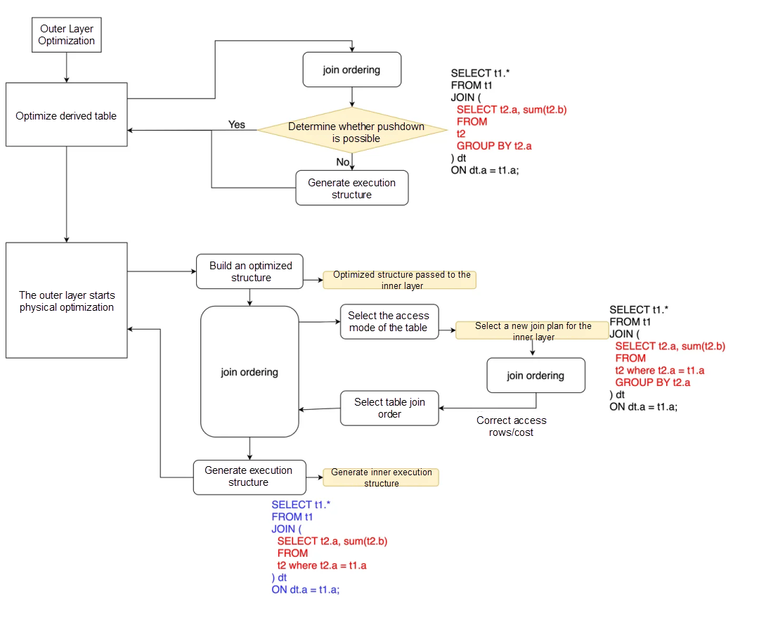
Obviously, this is a transformation that needs to be determined based on cost. Although the implementation is complex, the idea is relatively simple:

1. During the inner layer optimization of the derived table:

Optimize the Join Ordering of the inner derived table to obtain the full materialized cost in the non-pushdown case.
Determine whether JPPD is suitable, mark it if it is suitable, and collect such potential candidates.

2. Return to the outer layer optimization process, based on the Join conditions of the candidate derived table, build the relevant optimization structure, and pass to the inner layer of the derived table to build the inner relevant optimization structure for the Join condition pushdown.

3. When the outer layer starts the Join Ordering enumeration, retain the original Join plan for the derived table to be pushed down, optimize the structure based on the new pushdown condition, and re-optimize the Join Ordering to see if the index corresponding to the pushdown condition can be selected. If the index is selected, the inner layer generates a suitable candidate plan. If the index is not selected, restore the original Join Plan.

4. If the index is selected, you can adjust the number of output rows and materialized cost in the outer layer of the derived table. This way, the derived table can continue to participate in the enumeration process of the outer layer.

5. In the optimal Join plan selected by the outer layer, if the new plan is pushed down for the derived table, the new cost-based optimization strategy is selected.

6. When the physical execution structure is built at the outer layer, the conditions are also pushed into the inner layer of the derived table to build the relevant execution structure, establish dependencies, and eliminate unnecessary group by conditions.

It may be clearer with a flowchart and an example:

It can be seen that during the Join Ordering process at the outer layer, the possible new Join Plans at the inner layer are enumerated repeatedly. This overhead is unacceptable if the inner layer query is relatively large. Therefore, a caching mechanism is also required for the inner layer plan. In cases where there are possible association tables and associative indexes at the outer layer, the optimal plan is retained. If the same dependency relationship is encountered later, even if the outer Join order changes during enumeration, the inner plan can still be reused.

At the same time, if the inner group by column can be completely covered by the Join condition pushdown, it ensures that for each row at the outer layer, the data selected at the inner layer belongs to the same group. This allows for the elimination of group by to avoid unnecessary grouping calculations. However, it is important to note that this premise requires the presence of an aggregation function. Without an aggregation function, the deduplication effect achieved through group by will be lost, resulting in incorrect results.

Actual Effect

We still take TPC-H Q17 as an example, using the data volume of 10s for serial execution, the original query is as follows:

EXPLAIN
SELECT SUM(l_extendedprice) / 7.0 AS avg_yearly
FROM lineitem
  JOIN part ON p_partkey = l_partkey
WHERE p_brand = 'Brand#34'
  AND p_container = 'MED BOX'
  AND l_quantity < (
    SELECT 0.2 * AVG(l_quantity)
    FROM lineitem
    WHERE l_partkey = p_partkey
);

The execution plan:

| -> Aggregate: sum(lineitem.L_EXTENDEDPRICE)
    -> Nested loop inner join  (cost=779599.70 rows=511050)
        -> Filter: ((part.P_CONTAINER = 'MED BOX') and (part.P_BRAND = 'Brand#34'))  (cost=217445.20 rows=19743)
            -> Table scan on part  (cost=217445.20 rows=1974262)
        -> Filter: (lineitem.L_QUANTITY < (select #2))  (cost=25.89 rows=26)
            -> Index lookup on lineitem using LINEITEM_FK2 (L_PARTKEY=part.P_PARTKEY)  (cost=25.89 rows=26)
            -> Select #2 (subquery in condition; dependent)
                -> Aggregate: avg(lineitem.L_QUANTITY)
                    -> Index lookup on lineitem using LINEITEM_FK2 (L_PARTKEY=part.P_PARTKEY)  (cost=28.47 rows=26)

As you can see, the inner layer executes each row of data in the outer lineitem. Although the index LINEITEM_FK2 is used, the execution method is fixed.

The execution time is 3.49s

If the conversion from scalar subqueries to derived tables is enabled separately, the plan is as follows:

| -> Aggregate: sum(lineitem.L_EXTENDEDPRICE)
    -> Nested loop inner join
        -> Nested loop inner join  (cost=722658.72 rows=511050)
            -> Filter: ((part.P_CONTAINER = 'MED BOX') and (part.P_BRAND = 'Brand#34'))  (cost=202430.95 rows=19743)
                -> Table scan on part  (cost=202430.95 rows=1974262)
            -> Index lookup on lineitem using LINEITEM_FK2 (L_PARTKEY=part.P_PARTKEY)  (cost=23.76 rows=26)
        -> Filter: (lineitem.L_QUANTITY < derived_1_2.Name_exp_1)
            -> Index lookup on derived_1_2 using <auto_key2> (Name_exp_2=part.P_PARTKEY)
                -> Materialize
                    -> Group aggregate: avg(lineitem.L_QUANTITY)
                        -> Index scan on lineitem using LINEITEM_FK2  (cost=5896444.53 rows=54300917)

As you can see, after the subquery is fully materialized, it is joined with the outer query in the following order: part -> lineitem -> dt

If the execution time is long, it will be killed halfway.

However, if you add the JPPD optimization, you can generate the optimal plan as generated at the beginning of the article:

| -> Aggregate: sum(lineitem.L_EXTENDEDPRICE)
    -> Nested loop inner join
        -> Nested loop inner join
            -> Invalidate materialized tables (row from part)  (cost=202430.95 rows=19743)
                -> Filter: ((part.P_CONTAINER = 'MED BOX') and (part.P_BRAND = 'Brand#34'))  (cost=202430.95 rows=19743)
                    -> Table scan on part  (cost=202430.95 rows=1974262)
            -> Index lookup on derived_1_2 using <auto_key2> (Name_exp_2=part.P_PARTKEY)
                -> Materialize (invalidate on row from part)
                    -> Group aggregate: avg(lineitem.L_QUANTITY)
                        -> Index lookup on lineitem using LINEITEM_FK2 (L_PARTKEY=part.P_PARTKEY)  (cost=9.06 rows=26)
        -> Filter: (lineitem.L_QUANTITY < derived_1_2.Name_exp_1)  (cost=6.47 rows=9)
            -> Index lookup on lineitem using LINEITEM_FK2 (L_PARTKEY=part.P_PARTKEY)  (cost=6.47 rows=26)

As you can see, the outer join condition L_PARTKEY=part.P_PARTKEY is pushed down. Then, a Lateral Join is performed on the part table first, and then a Lineitem Join is performed on the part table, which is consistent with the expectation.

The execution time is 1.05s.

The time taken by online customers has been reduced from more than 60s to 0.5s. As we can see, the effect is obvious.

Summary

You may have a question about TPC-H Q17. The transformation we discussed is not necessarily better on its own, and the combination with JPPD can produce the optimal plan. However, it cannot be enabled by default. This may seem contradictory. However, this is the problem that our other important work, Cost-based query transformation, aims to solve.

The core of CBQT is to establish an enumeration framework. Within this framework, various transformation rules can be added to the codebase without being fixed. The completion of each transformation is determined based on cost, and the correlation between transformations is considered. This allows for the application of some transformations to each other and enables repetition. At the same time, we aim to minimize the additional overhead caused by repeated optimization, such as re-estimating statistics and re-optimizing query blocks. This helps us achieve a reasonable tradeoff between time, space, and plan optimality..

The development of the optimizer is an ongoing accumulation process. Although each feature may seem to be considered on a case-by-case basis, gradual accumulation will eventually lead to qualitative changes. Our goal is to delve deeper into each feature based on customer needs, apply them to as many scenarios as possible, and achieve the best possible results.

Free Tier & Special Offers of Alibaba Cloud Database Products: https://www.alibabacloud.com/product/databases

Community

About Database Kernel | PolarDB Optimizer Query Transformation - Join Condition Pushdown

Introduction

Preface

Join Predicate Pushdown

Applicable Conditions

Income Condition

Solutions

Actual Effect

Summary

Read previous post:

Read next post:

ApsaraDB

You may also like

Comments

ApsaraDB

Related Products

PolarDB for PostgreSQL

PolarDB for Xscale

PolarDB for MySQL

Database for FinTech Solution