MaxCompute：Python SDK樣本：DataFrame

假設已經存在三張表，分別是pyodps_ml_100k_movies（電影相關的資料）、pyodps_ml_100k_users（使用者相關的資料）和pyodps_ml_100k_ratings（評分有關的資料）。

1. 首先建立MaxCompute的入口對象。

   import os
   from odps import ODPS
   # 確保 ALIBABA_CLOUD_ACCESS_KEY_ID 環境變數設定為使用者 Access Key ID，
   # ALIBABA_CLOUD_ACCESS_KEY_SECRET 環境變數設定為使用者 Access Key Secret，
   # 不建議直接使用 Access Key ID / Access Key Secret 字串
   o = ODPS(
       os.getenv('ALIBABA_CLOUD_ACCESS_KEY_ID'),
       os.getenv('ALIBABA_CLOUD_ACCESS_KEY_SECRET'),
       project='your-default-project',
       endpoint='your-end-point',
   )

2. 傳入Table對象，建立DataFrame對象users。

   from odps.df import DataFrame
   users = DataFrame(o.get_table('pyodps_ml_100k_users'))

3. 對DataFrame對象可以執行如下操作：

   • 通過dtypes屬性可以查看DataFrame的欄位和類型，如下所示。

     users.dtypes

   • 通過head方法，可以擷取前N條資料，方便快速預覽資料。

     users.head(10)

     返回結果如下。

     -	user_id	age	sex	occupation	zip_code
     0	1	24	M	technician	85711
     1	2	53	F	other	94043
     2	3	23	M	writer	32067
     3	4	24	M	technician	43537
     4	5	33	F	other	15213
     5	6	42	M	executive	98101
     6	7	57	M	administrator	91344
     7	8	36	M	administrator	05201
     8	9	29	M	student	01002
     9	10	53	M	lawyer	90703

   • 對欄位進行篩選。

     • 篩選部分欄位。

       users[['user_id', 'age']].head(5)

       返回結果如下。

       -	user_id	age
       0	1	24
       1	2	53
       2	3	23
       3	4	24
       4	5	33

     • 排除個別欄位，如下所示。

       >>> users.exclude('zip_code', 'age').head(5)

       返回結果如下。

       -	user_id	sex	occupation
       0	1	M	technician
       1	2	F	other
       2	3	M	writer
       3	4	M	technician
       4	5	F	other

     • 排除掉一些欄位的同時，通過計算得到一些新的列。例如，將sex為M設定為True，否則設定為False，並將此列取名為sex_bool。如下所示。

       >>> users.select(users.exclude('zip_code', 'sex'), sex_bool=users.sex == 'M').head(5)

       返回結果如下。

       -	user_id	age	occupation	sex_bool
       0	1	24	technician	True
       1	2	53	other	False
       2	3	23	writer	True
       3	4	24	technician	True
       4	5	33	other	False

   • 查詢年齡在20~25歲之間的人數，如下所示。

     >>> users.age.between(20, 25).count().rename('count')
     943

   • 查詢男女使用者的數量。

     >>> users.groupby(users.sex).count()

     返回結果如下。

     -	sex	count
     0	F	273
     1	M	670

   • 將使用者按職業劃分，從高到底，擷取人數最多的前10個職業。

     >>> df = users.groupby('occupation').agg(count=users['occupation'].count())
     >>> df.sort(df['count'], ascending=False)[:10]

     返回結果如下。

     -	occupation	count
     0	student	196
     1	other	105
     2	educator	95
     3	administrator	79
     4	engineer	67
     5	programmer	66
     6	librarian	51
     7	writer	45
     8	executive	32
     9	scientist	31

     DataFrame API提供了value_counts方法來快速達到同樣的目的。

     >>> users.occupation.value_counts()[:10]

     返回結果如下。

     -	occupation	count
     0	student	196
     1	other	105
     2	educator	95
     3	administrator	79
     4	engineer	67
     5	programmer	66
     6	librarian	51
     7	writer	45
     8	executive	32
     9	scientist	31

   • 使用更直觀的圖來查看這份資料。

      %matplotlib inline

   • 使用橫向的柱狀圖來可視化。

     users['occupation'].value_counts().plot(kind='barh', x='occupation', ylabel='prefession')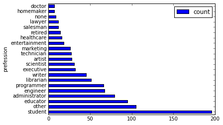

     

   • 使用長條圖來可視化。將年齡分成30組，查看各年齡分布的長條圖，如下所示。

     >>> users.age.hist(bins=30, title="Distribution of users' ages", xlabel='age', ylabel='count of users')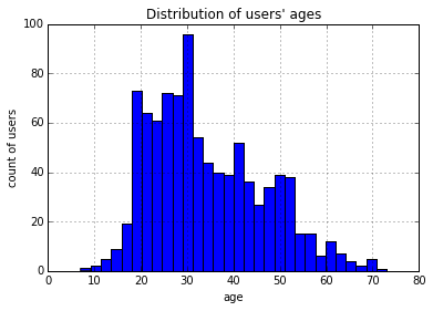

     

   • 使用JOIN將三張表進行聯合後，儲存成一張新的表。

     movies = DataFrame(o.get_table('pyodps_ml_100k_movies'))
     ratings = DataFrame(o.get_table('pyodps_ml_100k_ratings'))
     o.delete_table('pyodps_ml_100k_lens', if_exists=True)
     lens = movies.join(ratings).join(users).persist('pyodps_ml_100k_lens')
     lens.dtypes

     結果如下。

     odps.Schema {
       movie_id                            int64
       title                               string
       release_date                        string
       video_release_date                  string
       imdb_url                            string
       user_id                             int64
       rating                              int64
       unix_timestamp                      int64
       age                                 int64
       sex                                 string
       occupation                          string
       zip_code                            string
     }

   • 把0~79歲的年齡，分成8個年齡段。

     labels = ['0-9', '10-19', '20-29', '30-39', '40-49', '50-59', '60-69', '70-79']
     cut_lens = lens[lens, lens.age.cut(range(0, 80, 10), right=False, labels=labels).rename('年齡分組')]

   • 取分組和年齡唯一的前10條資料來進行查看。

     >>> cut_lens['年齡分組', 'age'].distinct()[:10]

     結果如下。

     -	年齡分組	age
     0	0-9	7
     1	10-19	10
     2	10-19	11
     3	10-19	13
     4	10-19	14
     5	10-19	15
     6	10-19	16
     7	10-19	17
     8	10-19	18
     9	10-19	19

   • 對各個年齡分組下，使用者的評分總數和評分均值進行查看，如下所示。

     cut_lens.groupby('年齡分組').agg(cut_lens.rating.count().rename('評分總數'), cut_lens.rating.mean().rename('評分均值'))

     結果如下。

     -	年齡分組	評分均值	評分總數
     0	0-9	3.767442	43
     1	10-19	3.486126	8181
     2	20-29	3.467333	39535
     3	30-39	3.554444	25696
     4	40-49	3.591772	15021
     5	50-59	3.635800	8704
     6	60-69	3.648875	2623
     7	70-79	3.649746	197