如何在Hologres中使用RuntimeFilter - Hologres

Hologres從V2.0版本開始支援Runtime Filter，在多表Join情境下自動最佳化Join過程的過濾行為，提升Join的查詢效能。本文為您介紹在Hologres中Runtime Filter的使用。

背景資訊

應用情境

Hologres從V2.0版本開始支援Runtime Filter，通常應用在多表（兩表及以上）Join的Hash Join情境，尤其是大表Join小表的情境中，無需手動設定，最佳化器和執行引擎會在查詢時自動最佳化Join過程的過濾行為，從而降低I/O開銷，以提升Join的查詢效能。

原理介紹

在瞭解Runtime Filter原理之前，需先瞭解Join過程。兩個表Join的SQL樣本如下：

select * from test1 join test2 on test1.x = test2.x;

其對應的執行計畫如下。

image..png

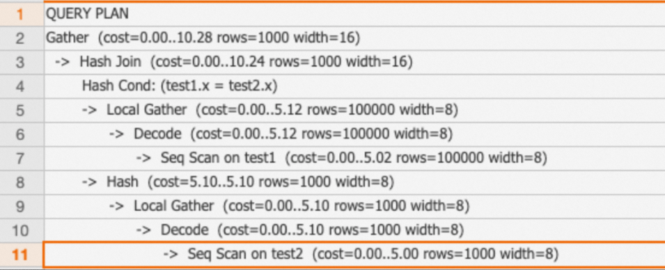
如上執行計畫，兩個表Join時，會通過test2表構建Hash表，然後匹配test1表的資料，最後返回結果。在這個過程中，Join時會涉及到兩個名詞：

build端：兩表（或者子查詢）做Hash Join時，其中一張表（子查詢）的資料會構建成Hash表，這一部分稱為build端，對應計劃裡的Hash節點。
probe端：Hash Join的另一邊，主要是讀取資料然後和build端的Hash表進行匹配，這一部分稱為probe端。

通常來說，在執行計畫正確的情況下，小表是build端，大表是probe端。

Runtime Filter的原理就是在HashJoin過程中，利用build端的資料分布，產生一個輕量的過濾器（filter），發送給probe端，對probe端的資料進行裁剪，從而減少probe端真正參與Hash Join以及網路傳輸的資料量，以此來提升Hash Join效能。

因此Runtime Filter更適用於大小表Join，且表資料量相差較大的情境，效能將會比普通Join有更多的提升。

使用限制和觸發條件

使用限制

僅Hologres V2.0及以上版本支援Runtime Filter。
僅支援Join條件中只有一個欄位，如果有多個欄位將不會觸發Runtime Filter。從Hologres V2.1版本開始，Runtime Filter支援多個欄位Join，如果多個Join欄位滿足觸發條件，也會觸發Runtime Filter。
僅4.0及以上版本支援 TopN Runtime Filter，用以提升單表 TopN 計算的情境的效能

觸發條件

Hologres本身支援高效能的Join，因此Runtime Filter會根據查詢條件在底層自動觸發，但是需要SQL滿足下述所有條件才能觸發：

probe端的資料量在100000行及以上。
掃描的資料量比例：build端 / probe端 <= 0.1（比例越小，越容易觸發Runtime Filter）。
Join出的資料量比例：build端 / probe端 <= 0.1（比例越小，越容易觸發Runtime Filter）。

Runtime Filter的類型

可以根據以下兩個維度對Runtime Filter進行分類。

按照Hash Join的probe端是否需要進行Shuffle，可分為Local和Global類型。
- Local類型：Hologres V2.0及以上版本支援。當Hash Join的probe端不需要Shuffle時，build端資料有如下三種情況，均可以使用Local類型的Runtime Filter：
  - build端和probe端的Join Key是同一種分布方式。
  - build端資料broadcast給probe端。
  - build端資料按照probe端資料的分布方式Shuffle給Probe端。
- Global類型：Hologres V2.2及以上版本支援。當probe端資料需要Shuffle時，Runtime Filter需要合并後才可以使用，這種情況需要使用Global類型的Runtime Filter。
Local類型的Runtime Filer僅可能減少資料掃描量以及參與Hash Join計算的資料量，Global類型的Runtime Filter由於probe端資料會Shuffle，在資料Shuffle之前做過濾還可以減少資料的網路傳輸量。類型都無需手動指定，引擎會自適應。
按照Filter類型，可分為Bloom Filter、In Filter和MinMAX Filter。
- Bloom Filter：Hologres V2.0及以上版本支援。Bloom Filter具有一定假陽性，導致少過濾一些資料，但其應用範圍廣，在build端資料量較多是仍能有較高的過濾效率，提升查詢效能。
- In Filter：Hologres V2.0及以上版本支援。In Filter在build端資料NDV（Number of Distinct Value，列的非重複值的個數）較小時使用，其會使用build端資料構建一個HashSet發送給probe端進行過濾，In Filter的優勢是可以過濾所有應該過濾的資料，且可以和Bitmap索引結合使用。
- MinMAX Filter：Hologres V2.0及以上版本支援。MinMAX Filter會根據build端資料得到最大值和最小值，發送給probe端做過濾，其優勢為可能根據中繼資料資訊直接過濾掉檔案或一個Batch的資料，減少I/O成本。
三種Filter類型無需您手動指定，Hologres會根據運行時Join情況自適應使用各種類型的Filter。

驗證Runtime Filter

如下樣本協助您更好地理解Runtime Filter。

樣本1：Join條件中只有1列，使用Local類型Runtime Filter

範例程式碼：

begin; 
create table test1(x int, y int);
call set_table_property('test1', 'distribution_key', 'x');

create table test2(x int, y int);
call set_table_property('test2', 'distribution_key', 'x');
end;

insert into test1 select t, t from generate_series(1, 100000) t;
insert into test2 select t, t from generate_series(1, 1000) t;
analyze test1;
analyze test2;

explain analyze select * from test1 join test2 on test1.x = test2.x;

執行計畫：
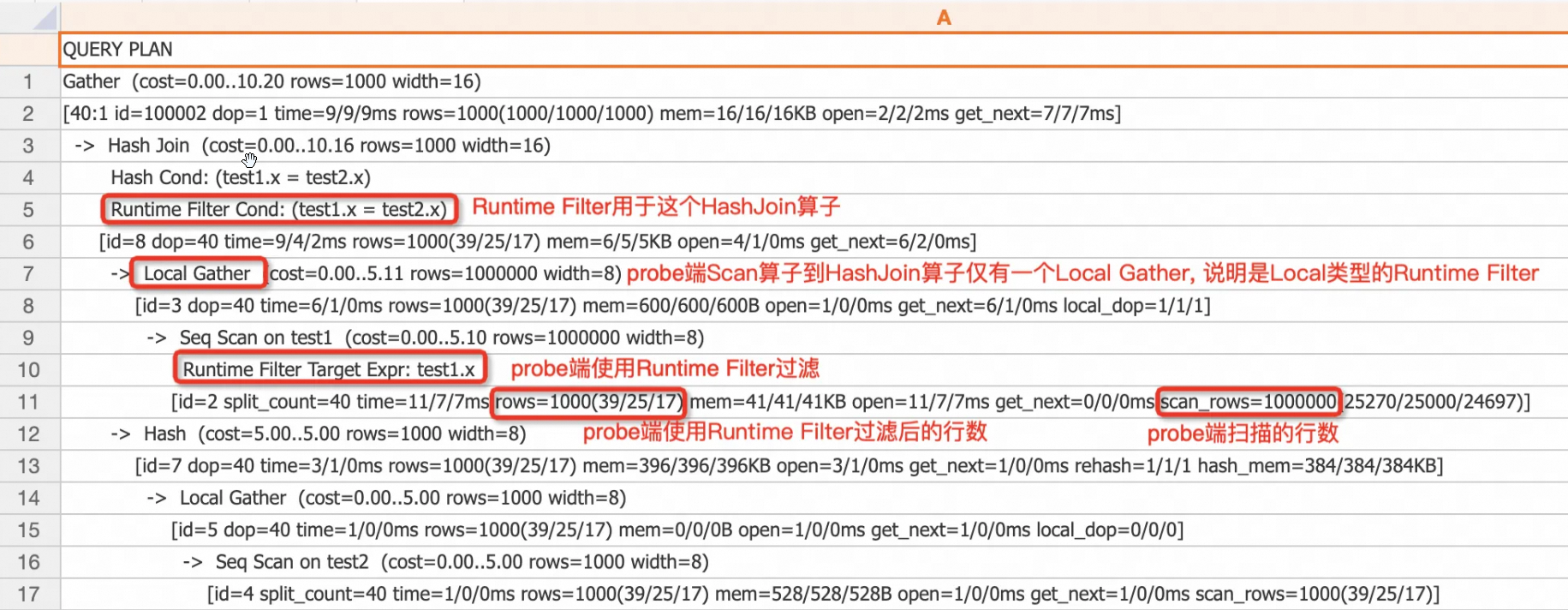
- test2表只有1000行，test1表有100000行，build端和probe端的資料量比例是0.01，小於0.1，且Join出來的資料量build端和probe端比例是0.01，小於0.1，滿足Runtime Filter的預設觸發條件，因此引擎會自動使用Runtime Filter。
- probe端的test1表有Runtime Filter Target Expr節點，表示probe端使用了Runtime Filter下推。
- probe端的scan_rows代表從儲存中讀取的資料，有100000行，rows代表使用Runtime Filter過濾後，scan運算元的行數，為1000行，可以從這兩個資料上看Runtime Filter的過濾效果。

樣本2：Join條件中有多列（Hologres V2.1版本支援），使用Local類型Runtime Filter

範例程式碼：

drop table if exists test1, test2;
begin;
create table test1(x int, y int);
create table test2(x int, y int);
end;
insert into test1 select t, t from generate_series(1, 1000000) t;
insert into test2 select t, t from generate_series(1, 1000) t;
analyze test1;
analyze test2;

explain analyze select * from test1 join test2 on test1.x = test2.x and test1.y = test2.y;

執行計畫：
- Join條件有多列，Runtime Filter也產生了多列。
- build端broadcast，可以使用Local類型的Runtime Filter。

樣本3：Global類型Runtime Filter支援Shuffle Join（Hologres V2.2版本支援）

範例程式碼：

SET hg_experimental_enable_result_cache = OFF;

drop table if exists test1, test2;
begin;
create table test1(x int, y int);
create table test2(x int, y int);
end;
insert into test1 select t, t from generate_series(1, 100000) t;
insert into test2 select t, t from generate_series(1, 1000) t;
analyze test1;
analyze test2;

explain analyze select * from test1 join test2 on test1.x = test2.x;

執行計畫：
從上述執行計畫可以看出，probe端資料被Shuffle到Hash Join運算元，引擎會自動使用Global Runtime Filter來加速查詢。

樣本4：In類型的Filter結合bitmap索引（Hologres V2.2版本支援）

範例程式碼：

set hg_experimental_enable_result_cache=off;

drop table if exists test1, test2;

begin;
create table test1(x text, y text);
call set_table_property('test1', 'distribution_key', 'x');
call set_table_property('test1', 'bitmap_columns', 'x');
call set_table_property('test1', 'dictionary_encoding_columns', '');

create table test2(x text, y text);
call set_table_property('test2', 'distribution_key', 'x');
end;

insert into test1 select t::text, t::text from generate_series(1, 10000000) t;

insert into test2 select t::text, t::text from generate_series(1, 50) t;

analyze test1;
analyze test2;

explain analyze select * from test1 join test2 on test1.x = test2.x;

執行計畫：
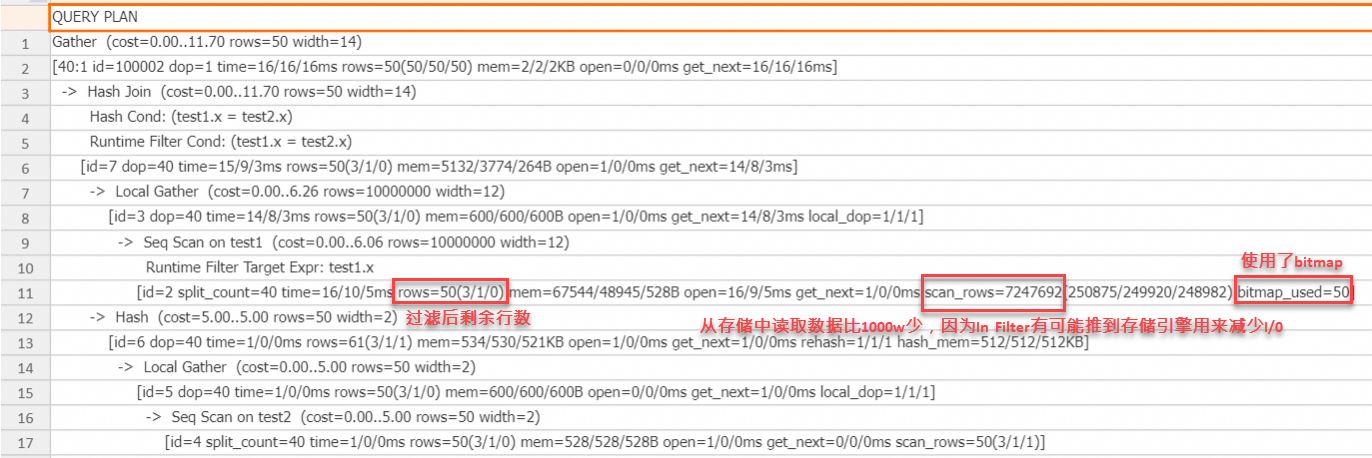
從上述執行計畫可以看出，在probe端的scan運算元上，使用了bitmap，因為In Filter可以精確過濾，因此過濾後還剩50行，scan運算元中的scan_rows為700多萬，比原始行數1000萬少，這是因為In Filter可以推到儲存引擎，有可能減少I/O成本，最終結果是從儲存引擎中讀取的資料變少了，In類型的Runtime Filter結合bitmap通常在Join Key為STRING類型時，有明顯作用。

樣本5：MinMax類型的Filter減少I/O（Hologres V2.2版本支援）

範例程式碼：

set hg_experimental_enable_result_cache=off;

drop table if exists test1, test2;

begin;
create table test1(x int, y int);
call set_table_property('test1', 'distribution_key', 'x');

create table test2(x int, y int);
call set_table_property('test2', 'distribution_key', 'x');
end;

insert into test1 select t::int, t::int from generate_series(1, 10000000) t;
insert into test2 select t::int, t::int from generate_series(1, 100000) t;

analyze test1;
analyze test2;

explain analyze select * from test1 join test2 on test1.x = test2.x;

執行計畫：
從上述執行計畫可以看出，probe端scan運算元從儲存引擎讀取的行數為32萬多，比原始行數1000萬少了很多，這是因為Runtime Filter被下推到儲存引擎，利用一個batch資料的meta資訊整批過濾資料，有可能大量減少I/O成本。通常在Join Key為數實值型別，且build端範圍範圍比probe端的範圍範圍小時，有明顯效果。

樣本6：TopN Runtime Filter（Hologres V4.0版本支援）

在 Hologres 中，資料是以分塊流式的方式進行處理的。因此，當 SQL 陳述式中包含 topN 運算元時，Hologres 並不會計算所有結果，而是會產生一個動態 Filter 來提前對資料進行過濾。

以下列SQL語句為例：

select o_orderkey from orders order by o_orderdate limit 5;

此 SQL 陳述式的執行計畫如下：

QUERY PLAN
Limit  (cost=0.00..116554.70 rows=0 width=8)
  ->  Sort  (cost=0.00..116554.70 rows=100 width=12)
        Sort Key: o_orderdate
      [id=6 dop=1 time=317/317/317ms rows=5(5/5/5) mem=1/1/1KB open=317/317/317ms get_next=0/0/0ms]
        ->  Gather  (cost=0.00..116554.25 rows=100 width=12)
            [20:1 id=100002 dop=1 time=317/317/317ms rows=100(100/100/100) mem=6/6/6KB open=0/0/0ms get_next=317/317/317ms * ]
              ->  Limit  (cost=0.00..116554.25 rows=0 width=12)
                    ->  Sort  (cost=0.00..116554.25 rows=150000000 width=12)
                          Sort Key: o_orderdate
                          Runtime Filter Sort Column: o_orderdate
                        [id=3 dop=20 time=318/282/258ms rows=100(5/5/5) mem=96/96/96KB open=318/282/258ms get_next=1/0/0ms]
                          ->  Local Gather  (cost=0.00..9.59 rows=150000000 width=12)
                              [id=2 dop=20 time=316/280/256ms rows=1372205(68691/68610/68498) mem=0/0/0B open=0/0/0ms get_next=316/280/256ms local_dop=1/1/1 * ]
                                ->  Seq Scan on orders  (cost=0.00..8.24 rows=150000000 width=12)
                                      Runtime Filter Target Expr: o_orderdate
                                    [id=1 split_count=20 time=286/249/222ms rows=1372205(68691/68610/68498) mem=179/179/179KB open=0/0/0ms get_next=286/249/222ms physical_reads=27074(1426/1353/1294) scan_rows=144867963(7324934/7243398/7172304)]
Query id:[1001003033996040311]
QE version: 2.0
Query Queue: init_warehouse.default_queue
======================cost======================
Total cost:[343] ms
Optimizer cost:[13] ms
Build execution plan cost:[0] ms
Init execution plan cost:[6] ms
Start query cost:[6] ms
- Queue cost: [0] ms
- Wait schema cost:[0] ms
- Lock query cost:[0] ms
- Create dataset reader cost:[0] ms
- Create split reader cost:[0] ms
Get result cost:[318] ms
- Get the first block cost:[318] ms
====================resource====================
Memory: total 7 MB. Worker stats: max 3 MB, avg 3 MB, min 3 MB, max memory worker id: 189*****.
CPU time: total 5167 ms. Worker stats: max 2610 ms, avg 2583 ms, min 2557 ms, max CPU time worker id: 189*****.
DAG CPU time stats: max 5165 ms, avg 2582 ms, min 0 ms, cnt 2, max CPU time dag id: 1.
Fragment CPU time stats: max 5137 ms, avg 1721 ms, min 0 ms, cnt 3, max CPU time fragment id: 2.
Ec wait time: total 90 ms. Worker stats: max 46 ms, max(max) 2 ms, avg 45 ms, min 44 ms, max ec wait time worker id: 189*****, max(max) ec wait time worker id: 189*****.
Physical read bytes: total 799 MB. Worker stats: max 400 MB, avg 399 MB, min 399 MB, max physical read bytes worker id: 189*****.
Read bytes: total 898 MB. Worker stats: max 450 MB, avg 449 MB, min 448 MB, max read bytes worker id: 189*****.
DAG instance count: total 3. Worker stats: max 2, avg 1, min 1, max DAG instance count worker id: 189*****.
Fragment instance count: total 41. Worker stats: max 21, avg 20, min 20, max fragment instance count worker id: 189*****.

沒有 TopN Filter 時，Scan 節點讀取 orders 表的每個資料區塊，並將它們傳給 TopN 節點。TopN 節點用堆排序維護當前已見資料中排名前 5 的行。

例如：

每個資料區塊約含 8192 行。處理完第一個塊後，TopN 就知道該塊中第 5 名的 o_orderdate。假設它是 1995-01-01。

Scan 節點在讀第二個塊時，就用 1995-01-01 作過濾條件。它只發送 o_orderdate ≤ 1995-01-01 的行給 TopN。閾值會動態更新。如果第二個塊中第 5 名的 o_orderdate 更小，TopN 就用這個新值替換舊閾值。

用 EXPLAIN 命令可查看最佳化器產生的 TopN Runtime Filter。

->  Limit  (cost=0.00..116554.25 rows=0 width=12)
  ->  Sort  (cost=0.00..116554.25 rows=150000000 width=12)
        Sort Key: o_orderdate
        Runtime Filter Sort Column: o_orderdate
      [id=3 dop=20 time=318/282/258ms rows=100(5/5/5) mem=96/96/96KB open=318/282/258ms get_next=1/0/0ms]

如上述例子所示：TopN 節點上會顯示 Runtime Filter Sort Column，表示這個 TopN 節點會產生一個 TopN Runtime Filter。