Job performance issues - Realtime Compute for Apache Flink

This topic covers common job performance issues.

How do I split operator nodes?
What are the Group Aggregate optimization techniques?
What are the TopN optimization techniques?
What are efficient deduplication solutions?
What should I note when using built-in functions?
How do I resolve low efficiency and backpressure during full-table read?
What do the color indicators in Status Durations for vertex subtasks mean in the job overview?
What is the RMI TCP Connection thread, and why does it use so much more CPU than other threads?
Why do Low Watermark, Watermark, and Task InputWatermark in the running topology show a time difference from the current time?
How do I troubleshoot job backpressure?
How do I troubleshoot high job latency?
How do I optimize Flink SQL jobs experiencing backpressure due to data hotspots?
How do I troubleshoot unstable upstream data consumption rates?

How do I split operator nodes?

In the Operation Center > Job O&M page, click the target job name. In the Deployment Details tab, under the Runtime Parameter Settings section, add the following code in Other Settings and save to apply.

pipeline.operator-chaining: 'false'

What are the Group Aggregate optimization techniques?

Enable MiniBatch (improves throughput)

MiniBatch buffers incoming data before triggering processing. This reduces State access frequency, increases throughput, and decreases output volume.

MiniBatch triggers micro-batch processing based on event messages inserted at your specified interval at the source.
- Scenarios
  
  Micro-batching trades slightly higher latency for significantly higher throughput. Do not enable it if you require ultra-low latency. For most aggregation scenarios, enabling MiniBatch greatly improves system performance.
- How to enable
  MiniBatch is disabled by default. To enable it, go to the Deployment Details tab of your target job, and in the Runtime Parameter Settings section under Other Settings, add the following code.
```
table.exec.mini-batch.enabled: true
table.exec.mini-batch.allow-latency: 5s
```
  The parameters are explained in the following table.
  
  Parameter
  
  Description
  
  table.exec.mini-batch.enabled
  
  Whether to enable mini-batch.
  
  table.exec.mini-batch.allow-latency
  
  Time interval between batch outputs.
Enable LocalGlobal (resolves common data hotspot issues)

The LocalGlobal mechanism uses LocalAgg to pre-aggregate skewed data, reducing hotspot pressure on GlobalAgg and improving overall performance.

LocalGlobal splits a single aggregate into two stages: Local and Global—similar to the Combine and Reduce phases in MapReduce. In the first stage, upstream nodes locally buffer and aggregate data (localAgg), emitting incremental accumulators. In the second stage, these accumulators are merged (Merge) to produce the final result (GlobalAgg).
- Scenarios
  
  Improves performance for standard aggregations (such as SUM, COUNT, MAX, MIN, and AVG) and resolves data hotspot issues in these scenarios.
- Limits
  LocalGlobal is enabled by default, but it has the following limitations:
  - MiniBatch must be enabled.
  - Your AggregateFunction must implement Merge.
- Verify that the change takes effect
  
  Check whether the generated topology contains nodes named GlobalGroupAggregate or LocalGroupAggregate.
Enable PartialFinal (resolves COUNT DISTINCT hotspot issues)

To address COUNT DISTINCT hotspots, you traditionally had to manually rewrite queries into two-stage aggregation (adding a modulo-based shuffling layer). Realtime Compute for Apache Flink now provides automatic COUNT DISTINCT shuffling via PartialFinal optimization—no manual rewriting needed.

LocalGlobal works well for standard aggregations but offers little benefit for COUNT DISTINCT. During local aggregation, distinct key deduplication rates remain low, so hotspots persist at the global node.
- Scenarios
  Use when COUNT DISTINCT fails to meet aggregation node performance requirements.
  Important
  
  Do not use PartialFinal optimization in Flink SQL that includes UDAFs.
  
  Avoid PartialFinal when data volume is small—it introduces unnecessary network shuffling and wastes resources.
- How to enable
  This feature is disabled by default. To enable it, on the Deployment Details tab of the target job, in the Runtime Parameter Settings section, enter the following code in the Other Configurations field.
```
table.optimizer.distinct-agg.split.enabled: true
```
- Verify that the changes are effective.
  
  Check whether the generated topology changes from a single aggregation stage to two stages.
Rewrite AGG WITH CASE WHEN as AGG WITH FILTER syntax (boosts performance for multiple COUNT DISTINCT scenarios)
If your job calculates UV across dimensions—such as total UV, mobile client UV, and PC UV—use standard AGG WITH FILTER syntax instead of CASE WHEN. The Realtime Compute SQL optimizer recognizes Filter parameters, allowing multiple COUNT DISTINCT operations on the same field to share State and reduce State I/O. Performance tests show this rewrite can double performance.
- Scenarios
  
  Significant performance gains occur when computing multiple COUNT DISTINCT results on the same field under different conditions.
- Original text
```
COUNT(distinct visitor_id) as UV1 , COUNT(distinct case when is_wireless='y' then visitor_id else null end) as UV2
```
- Optimized syntax
```
COUNT(distinct visitor_id) as UV1 , COUNT(distinct visitor_id) filter (where is_wireless='y') as UV2
```

What are the TopN optimization techniques?

TopN algorithms
If TopN input is an append-only stream (for example, from SLS), only one algorithm is available: AppendRank. If input is an update stream (for example, after AGG or JOIN), two algorithms are available, ranked from highest to lowest performance: UpdateFastRank and RetractRank. Algorithm names appear in topology node labels.
- AppendRank: Only supported for append-only streams.
- UpdateFastRank: Optimal for update streams.
- RetractRank: Fallback algorithm for update streams. Lower performance. In some cases, it can be optimized to UpdateFastRank.
To optimize RetractRank into UpdateFastRank, three conditions must be met:
- Input stream must be an update stream.
- Input stream must include Primary Key information—for example, after a GROUP BY aggregation.
- Sort fields must update monotonically in the opposite direction of sorting. For example, ORDER BY COUNT, COUNT_DISTINCT, or SUM (positive values) DESC.
To ensure UpdateFastRank is used with ORDER BY SUM DESC, add a filter condition guaranteeing total_fee is positive.
```
insert
  into print_test
SELECT
  cate_id,
  seller_id,
  stat_date,
  pay_ord_amt  -- Omit rownum to reduce sink table output.
FROM (
    SELECT
      *,
      ROW_NUMBER () OVER (
        PARTITION BY cate_id,
        stat_date  -- Include a time field to prevent data corruption from State TTL.
        ORDER
          BY pay_ord_amt DESC
      ) as rownum  -- Sort by upstream sum result.
    FROM (
        SELECT
          cate_id,
          seller_id,
          stat_date,
          -- Critical: Declare all SUM inputs as positive, ensuring monotonic increase.
          -- This allows TopN to use the optimized algorithm and fetch only top 100 records.
          sum (total_fee) filter (
            where
              total_fee >= 0
          ) as pay_ord_amt
        FROM
          random_test
        WHERE
          total_fee >= 0
        GROUP
          BY cate_name,
          seller_id,
          stat_date,
          cate_id
      ) a
    ) WHERE
      rownum <= 100;
```
TopN optimization methods
- No Ranking Output Optimization
  
  If your TopN output does not need to display rownum values, omit them and sort only once in the frontend. This drastically reduces sink table output volume. For details, see Top-N.
- Increase TopN cache size
  TopN uses a State Cache layer to improve State access efficiency. Cache hit rate is calculated as follows.
```
cache_hit = cache_size*parallelism/top_n/partition_key_num
```
  For example, with Top100, cache size 10,000, parallelism 50, and 100,000 partition keys, the hit rate is only 10000*50/100/100000=5%. Low hit rates cause most requests to hit disk-based State, creating glitches in state seek metrics and severely degrading performance.
  
  When partition key cardinality is very high, increase TopN cache size and heap memory accordingly. For details, see Configure job deployment settings.
```
table.exec.rank.topn-cache-size: 200000
```
  The default cache size is 10,000. Increasing it to 200,000 raises theoretical hit rate to 200000*50/100/100000 = 100%.
- Include a time-based field in PartitionBy
  
  For daily rankings, include a Day field. Without it, State TTL may corrupt final TopN results.

What are efficient deduplication solutions?

Source data in Realtime Compute for Apache Flink sometimes contains duplicates. Users frequently request deduplication. Realtime Compute supports two strategies: keep first row (Deduplicate Keep FirstRow) and keep last row (Deduplicate Keep LastRow).

Syntax

SQL lacks direct deduplication syntax, so we use ROW_NUMBER OVER WINDOW to implement it. Deduplication is essentially a special form of TopN.

SELECT *
FROM (
   SELECT *,
    ROW_NUMBER() OVER (PARTITION BY col1[, col2..]
     ORDER BY timeAttributeCol [asc|desc]) AS rownum
   FROM table_name)
WHERE rownum = 1

Parameter	Description
ROW_NUMBER()	Window function that assigns row numbers starting from 1.
PARTITION BY col1[, col2..]	Optional. Columns defining partitions (deduplication keys).
ORDER BY timeAttributeCol [asc\|desc])	Column used for sorting. Must be a time attribute field (Proctime or Rowtime). Use ascending order for Keep FirstRow or descending for Keep LastRow.
rownum	Only `rownum=1` or `rownum<=1` is supported.

As shown above, deduplication requires two query layers:

Use ROW_NUMBER() to sort data by time attribute and assign ranks.
- If the sort field is Proctime, Flink deduplicates by system time, producing non-deterministic results.
- If the sort field is Rowtime, Flink deduplicates by business time, producing deterministic results.
Filter by rank to keep only the first row, achieving deduplication.
The data can be sorted in ascending or descending order by the time column:
- Deduplicate Keep FirstRow: Ascending order, keep first row.
- Deduplicate Keep LastRow: Descending order, keep first row.

Deduplicate Keep FirstRow
This strategy keeps the first occurrence of each key and discards subsequent duplicates. It stores only key data in State, offering better performance. Example:
```
SELECT *
FROM (
  SELECT *,
    ROW_NUMBER() OVER (PARTITION BY b ORDER BY proctime) as rowNum
  FROM T
)
WHERE rowNum = 1
```
This example deduplicates table T by field b, keeping the first row by system time. Here, proctime is a Processing Time attribute field in source table T. When deduplicating by system time, you can simplify proctime to the proctime() function call and omit explicit field declaration.
Deduplicate Keep LastRow
This strategy keeps the last occurrence of each key. It performs slightly better than LAST_VALUE. Example:
```
SELECT *
FROM (
  SELECT *,
    ROW_NUMBER() OVER (PARTITION BY b, d ORDER BY rowtime DESC) as rowNum
  FROM T
)
WHERE rowNum = 1
```
This example deduplicates table T by fields b and d, keeping the last row by business time. Here, rowtime is an Event Time attribute field in source table T.

What should I note when using built-in functions?

Replace user-defined functions with built-in functions

Realtime Compute continuously optimizes built-in functions. Prefer them over user-defined functions. Key optimizations include the following:
- Reduced serialization and deserialization overhead.
- Direct byte-level operations.
Use single-character separators in KEY VALUE functions

KEY VALUE signature: KEYVALUE(content, keyValueSplit, keySplit, keyName). When keyValueSplit and keySplit are single characters (such as colon ":" or comma ","), the system uses an optimized algorithm to directly locate keyName in binary data without splitting the entire content—improving performance by about 30%.
LIKE operation notes
- For StartWith, use LIKE 'xxx%'.
- For EndWith, use LIKE '%xxx'.
- For Contains, use LIKE '%xxx%'.
- For Equals, use LIKE 'xxx', equivalent to str = 'xxx'.
- To match underscore (_), escape it: LIKE '%seller/_id%' ESCAPE '/'. Underscore (_) is a single-character wildcard in SQL. Without escaping, LIKE '%seller_id%' matches seller_id, seller#id, sellerxid, and seller1id, causing incorrect results.
Avoid regular expression functions (REGEXP)
Regular expressions are extremely expensive—often 100× slower than basic arithmetic—and can enter infinite loops under certain conditions, blocking jobs. See Regex execution is too slow. Prefer LIKE. Regular expression functions include the following:
- REGEXP
- REGEXP_REPLACE

How do I resolve low efficiency and backpressure during full-table read?

Backpressure may stem from slow downstream processing. First, check for downstream backpressure. If present, resolve it using one of the following:

Increase concurrency.
Enable aggregation optimizations such as minibatch (for downstream aggregate nodes).

What do the color indicators in Status Durations for vertex subtasks mean in the job overview?

In the job Overview page, click an operator node and select the SubTasks tab to view colored duration badges in the Status Durations column.

Status Durations shows time spent by vertex subtasks in each phase. Color meanings are:

: CREATED
: SCHEDULED
: DEPLOYING
: INITIALIZING
: RUNNING

What is the RMI TCP Connection thread, and why does it use so much more CPU than other threads?

In the thread monitoring list sorted by CPU usage, the RMI TCP Connection(62)-172.25.240.255 thread shows RUNNABLE status with 82.3% CPU usage—much higher than kafkaRequestSource threads (16.9%–26.4% CPU, mostly TIMED_WAITING).

RMI TCP Connection threads belong to Java’s built-in RMI (Remote Method Invocation) framework and handle remote method calls. CPU usage fluctuates dynamically. Short-term spikes do not indicate sustained high load. Observe CPU usage over time. Flame graph analysis (below) shows RMI threads consume almost no CPU.

Why do Low Watermark, Watermark, and Task InputWatermark in the running topology show a time difference from the current time?

Reason 1: Source table Watermark declared with TIMESTAMP_LTZ (TIMESTAMP(p) WITH LOCAL TIME ZONE) causes time differences.

The following examples compare Watermark behavior with TIMESTAMP_LTZ versus TIMESTAMP types.

Source table Watermark uses TIMESTAMP_LTZ type.

CREATE TEMPORARY TABLE s1 (
  a INT,
  b INT,
  ts as CURRENT_TIMESTAMP,-- CURRENT_TIMESTAMP generates TIMESTAMP_LTZ.
  WATERMARK FOR ts AS ts - INTERVAL '5' SECOND 
) WITH (
  'connector'='datagen',
  'rows-per-second'='1',
  'fields.b.kind'='random','fields.b.min'='0','fields.b.max'='10'
);
CREATE TEMPORARY TABLE t1 (
  k INT,
  ts_ltz timestamp_ltz(3),
  cnt BIGINT
) WITH ('connector' = 'print');
-- Output results.
INSERT INTO t1
SELECT b, window_start, COUNT(*) FROM
TABLE(
    TUMBLE(TABLE s1, DESCRIPTOR(ts), INTERVAL '5' SECOND))
GROUP BY b, window_start, window_end;

Note

Legacy Window syntax produces identical results to TVF Window (Table-Valued Function). Legacy syntax example:

SELECT b, TUMBLE_END(ts, INTERVAL '5' SECOND), COUNT(*) FROM s1 GROUP BY TUMBLE(ts, INTERVAL '5' SECOND), b;

After deploying and running the job in the Realtime Compute development console, observe an 8-hour time difference between Watermark and current time (using UTC+8 as reference).

Watermark & Low Watermark

In the Flink job monitoring UI Watermarks tab, SubTask 0 shows Watermark value 1706778525521, corresponding to Datetime of Watermark Timestamp 02-01 09:08:45. Job start time was 02-01 17:03:04—an ~8-hour gap. The operator panel on the left shows identical Low Watermark 02-01 09:08:45.
Task InputWatermark

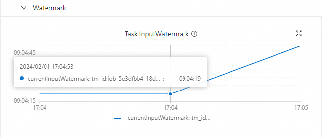
Source table Watermark uses TIMESTAMP (TIMESTAMP(p) WITHOUT TIME ZONE) type.

CREATE TEMPORARY TABLE s1 (
  a INT,
  b INT,
  -- Simulate TIMESTAMP without timezone, starting at 2024-01-31 01:00:00 and incrementing by second.
  ts as TIMESTAMPADD(SECOND, a, TIMESTAMP '2024-01-31 01:00:00'),
  WATERMARK FOR ts AS ts - INTERVAL '5' SECOND 
) WITH (
  'connector'='datagen',
  'rows-per-second'='1',
  'fields.a.kind'='sequence','fields.a.start'='0','fields.a.end'='100000',
  'fields.b.kind'='random','fields.b.min'='0','fields.b.max'='10'
);
CREATE TEMPORARY TABLE t1 (
  k INT,
  ts_ltz timestamp_ltz(3),
  cnt BIGINT
) WITH ('connector' = 'print');
-- Output results.
INSERT INTO t1
SELECT b, window_start, COUNT(*) FROM
TABLE(
    TUMBLE(TABLE s1, DESCRIPTOR(ts), INTERVAL '5' SECOND))
GROUP BY b, window_start, window_end;

After deploying and running in the Realtime Compute development console, Watermark aligns with current time (specifically, simulated data time)—no time difference.

Watermark & Low Watermark

In the Flink Web UI task details, select an operator (e.g., GlobalWindowAggregate). The left operator info panel shows Low Watermark (e.g., 01-31 01:03:49). Switch to the Watermarks tab on the right to view SubTask Watermark values and timestamps—both times match.
Task InputWatermark

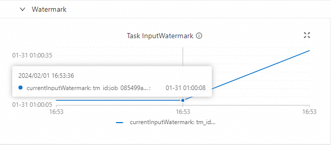
Reason 2: Timezone difference between Realtime Compute development console and Apache Flink UI.

The Realtime Compute development console displays times in UTC+0. Apache Flink UI uses the browser’s local timezone. Using UTC+8 (Beijing time) as reference, the Realtime Compute development console shows times 8 hours behind Apache Flink UI.
- Realtime Compute development console
  
  In the Job O&M page topology, Watermark times display in UTC+0. For example, when event time is Beijing time 2024/1/31 09:01:34 AM, the console shows 2024/1/31 01:01:34 AM.
  
  Watermark-related monitoring metrics in the product console also use UTC+0—8 hours behind Beijing time.
- Apache Flink UI
  
  In the Apache Flink Web UI, select an operator node (e.g., GlobalWindowAggregate) in the job topology and switch to the Watermarks tab. View SubTask Watermark values and corresponding event times. For example, Low Watermark 1706662894000 corresponds to Datetime of Watermark Timestamp 2024/1/31 09:01:34 AM. This is event time, not processing time—so differences from system time are normal.

How to troubleshoot job backpressure issues?

In the Job O&M page, click the target job name to open the Overview tab.
Check Busy and BackPressure to locate backpressure.

Redder Busy indicators mean heavier task load. Darker BackPressure indicators mean stronger backpressure impact.

For example, if upstream operator Backpressured (max) is 99%, middle operator Busy (max) is 100% (red highlight), and downstream operator Busy (max) is only 7%, the bottleneck is the middle operator—optimize it.
Click the backpressured operator.
In the BackPressure tab, check SubTask backpressure status.

If Back Pressure Status is green OK, and the table shows SubTasks 0–7 with Backpressured / Idle / Busy as 0%, 0%, N/A and all states OK, the job has no backpressure.

How do I troubleshoot issues with excessive job latency?

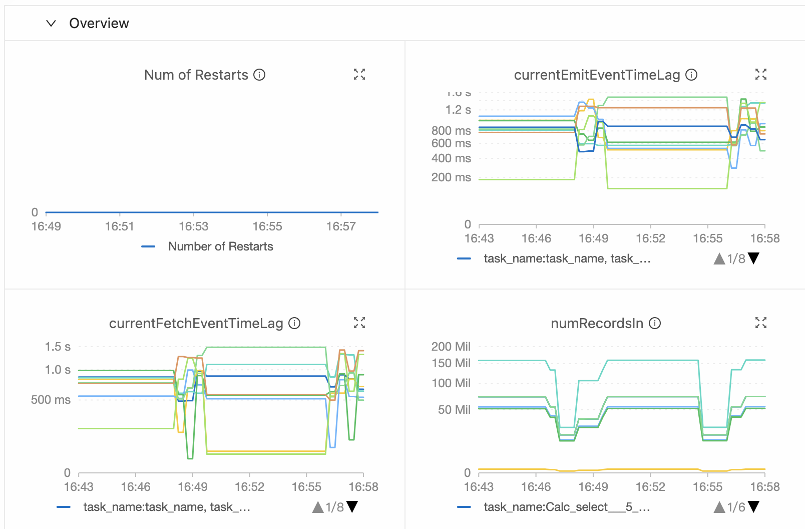
In the Job O&M page, check the Monitoring and Alerts or Data Curves tab for currentEmitEventTimeLag and currentFetchEventTimeLag metrics:

If currentEmitEventTimeLag is high, the job has delays in data fetching or processing. Check operator performance.
If currentFetchEventTimeLag is high, delays stem from data fetching or upstream system processing. Investigate network I/O and upstream systems.

Note

When upstream factors cause high latency, both metrics increase simultaneously.

How do you optimize a Flink SQL job when data skew causes backpressure?

When backpressure stems from data hotspots (confirmed via Subtask analysis), use these optimizations:

Enable LocalGlobal (resolves common data hotspot issues)

The LocalGlobal mechanism uses LocalAgg to pre-aggregate skewed data, reducing hotspot pressure on GlobalAgg and improving overall performance.

LocalGlobal splits a single aggregate into two stages: Local and Global—similar to the Combine and Reduce phases in MapReduce. In the first stage, upstream nodes locally buffer and aggregate data (localAgg), emitting incremental accumulators. In the second stage, these accumulators are merged (Merge) to produce the final result (GlobalAgg).
- Scenarios
  
  Improves performance for standard aggregations (such as SUM, COUNT, MAX, MIN, and AVG) and resolves data hotspot issues in these scenarios.
- Limits
  LocalGlobal is enabled by default, but the following limitations apply:
  - MiniBatch must be enabled.
  - Your AggregateFunction must implement Merge.
- Checking the status
  
  Check whether the generated topology contains nodes named GlobalGroupAggregate or LocalGroupAggregate.
Enable PartialFinal (resolves COUNT DISTINCT hotspot issues)

To address COUNT DISTINCT hotspots, you traditionally had to manually rewrite queries into two-stage aggregation (adding a modulo-based shuffling layer). Realtime Compute for Apache Flink now provides automatic COUNT DISTINCT shuffling via PartialFinal optimization—no manual rewriting needed.

LocalGlobal works well for standard aggregations but offers little benefit for COUNT DISTINCT. During local aggregation, distinct key deduplication rates remain low, so hotspots persist at the global node.
- Scenarios
  Use when COUNT DISTINCT fails to meet aggregation node performance requirements.
  Important
  
  Do not use PartialFinal optimization in Flink SQL that includes UDAFs.
  
  Avoid PartialFinal when data volume is small—it introduces unnecessary network shuffling and wastes resources.
- How to enable
  By default, this feature is disabled. To enable this feature, on the Deployment Details tab for the target job, enter the following code in the Other Configurations section of the Runtime Parameter Settings area.
```
table.optimizer.distinct-agg.split.enabled: true
```
- Verify the effectiveness
  
  Check whether the generated topology changes from a single aggregation stage to two stages.

How do I troubleshoot unstable speed of consuming input data?

Possible causes and solutions:

Upstream data production pattern mismatches current processing speed.

Analyze upstream data generation patterns to align production and processing rates.
Job experiences backpressure.

Check for backpressure affecting upstream consumption. If your job shows only one node, add pipeline.operator-chaining: 'false', restart the job to split the operator chain, and identify any backpressured nodes impacting consumption rate.
Abnormal I/O rate.

Review Flink’s data input and consumption rate curves at the relevant time to determine if I/O is the cause.
Abnormal consumption rate.

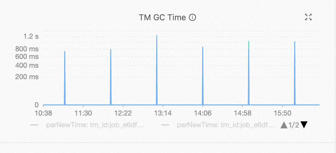
Check if consumption rate fluctuations align with Garbage Collection (GC) events. If they do, inspect TM node memory usage.

Parameter	Description
table.exec.mini-batch.enabled	Whether to enable mini-batch.
table.exec.mini-batch.allow-latency	Time interval between batch outputs.