PostgreSQL: Stock Price Prediction Using Multiple Linear Regression Analysis

By digoal

Background

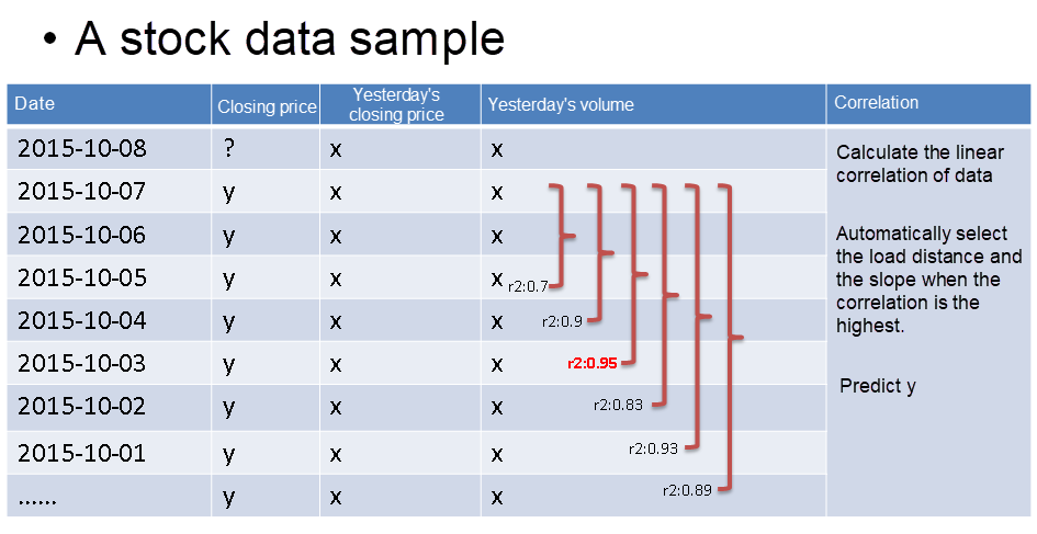
The previous two articles introduced one-dimensional linear regression for stock price prediction, so only one independent variable was used. It is inaccurate to predict today's closing price based on yesterday’s closing price using a single element unless the results primarily depend on independent variables.

Multiple regression predicts more accurate results when the results depend on more than one variable. For example, you can use ternary regression to predict the next day's closing price based on yesterday's volume, closing price, and opening price.

In PostgreSQL, you can implement multiple linear regression using the MADlib library.

Example:

The Formula of P-variables Linear Regression:

y1=b0+b1x11+b2x12+…+bpx1p+ε1  
y2=b0+b1x21+b2x22+…+bpx2p+ε2  
………………

1) Obtain intercept and slope.

2) Predict yn.

yn=b0+b1xn1+b2xn2+…+bpxnp+εn

R Formula:

lm(y: 收盘价 ~ x1: 昨日收盘价 + x2: 昨日成交量, $DATA)

Practical example: http://doc.madlib.net/latest/group__grp__linreg.html

Create an input data set.  
CREATE TABLE houses (id INT, tax INT, bedroom INT, bath FLOAT, price INT,  
            size INT, lot INT);  
COPY houses FROM STDIN WITH DELIMITER '|';  
  1 |  590 |       2 |    1 |  50000 |  770 | 22100  
  2 | 1050 |       3 |    2 |  85000 | 1410 | 12000  
  3 |   20 |       3 |    1 |  22500 | 1060 |  3500  
  4 |  870 |       2 |    2 |  90000 | 1300 | 17500  
  5 | 1320 |       3 |    2 | 133000 | 1500 | 30000  
  6 | 1350 |       2 |    1 |  90500 |  820 | 25700  
  7 | 2790 |       3 |  2.5 | 260000 | 2130 | 25000  
  8 |  680 |       2 |    1 | 142500 | 1170 | 22000  
  9 | 1840 |       3 |    2 | 160000 | 1500 | 19000  
 10 | 3680 |       4 |    2 | 240000 | 2790 | 20000  
 11 | 1660 |       3 |    1 |  87000 | 1030 | 17500  
 12 | 1620 |       3 |    2 | 118600 | 1250 | 20000  
 13 | 3100 |       3 |    2 | 140000 | 1760 | 38000  
 14 | 2070 |       2 |    3 | 148000 | 1550 | 14000  
 15 |  650 |       3 |  1.5 |  65000 | 1450 | 12000  
\.

Prediction model:

linregr_train( source_table,  
               out_table,  
               dependent_varname,  
               independent_varname,  
               grouping_cols,  -- 可选  
               heteroskedasticity_option  -- 可选  
             )  
  
Train a regression model. First, a single regression for all the data.

The “houses” contain historical data, including independent variables and dependent variables. Price is a dependent variable, and tax, bath, and size are independent variables. This is so-called ternary linear regression.

The “houses_linregr” stores the linear regression statistics, including correlation, R2, standard deviation, P value, etc.

SELECT madlib.linregr_train( 'houses',  
                             'houses_linregr',  
                             'price',  
                             'ARRAY[1, tax, bath, size]'  
                           );

It is feasible to add grouping fields when group predictions based on source data are required.

Generate three output models, one for each value of "bedroom".  
  
SELECT madlib.linregr_train( 'houses',  
                             'houses_linregr_bedroom',  
                             'price',  
                             'ARRAY[1, tax, bath, size]',  
                             'bedroom'  
                           );  
  
Examine the resulting models.  
  
-- Set extended display on for easier reading of output  
  
\x ON  
  
SELECT * FROM houses_linregr;  
Result:  
-[ RECORD 1 ]+---------------------------------------------------------------------------  
coef         | {-12849.4168959872,28.9613922651765,10181.6290712648,50.516894915354}  
r2           | 0.768577580597443  
std_err      | {33453.0344331391,15.8992104963997,19437.7710925923,32.928023174087}  
t_stats      | {-0.38410317968819,1.82156166004184,0.523806408809133,1.53416118083605}  
p_values     | {0.708223134615422,0.0958005827189772,0.610804093526536,0.153235085548186}  
condition_no | 9002.50457085737

The value of R2 is 0.76, meaning its correlation is poor. So, dynamic data segment computing mentioned earlier is needed for good correlation.

View the results grouped by bedroom.  
SELECT * FROM houses_linregr_bedroom;  
Result:  
-[ RECORD 1 ]+--------------------------------------------------------------------------  
bedroom      | 2  
coef         | {-84242.0345406597,55.4430144648696,-78966.9753675319,225.611910021192}  
r2           | 0.968809546465313  
std_err      | {35018.9991665742,19.5731125320686,23036.8071292552,49.0448678148784}  
t_stats      | {-2.40560942761235,2.83261103077151,-3.42786111480046,4.60011251070697}  
p_values     | {0.250804617665239,0.21605133377602,0.180704400437373,0.136272031474122}  
condition_no | 10086.1048721726  
-[ RECORD 2 ]+--------------------------------------------------------------------------  
bedroom      | 4  
coef         | {0.0112536020318378,41.4132554771633,0.0225072040636757,31.3975496688276}  
r2           | 1  
std_err      | {0,0,0,0}  
t_stats      | {Infinity,Infinity,Infinity,Infinity}  
p_values     |  
condition_no | Infinity  
-[ RECORD 3 ]+--------------------------------------------------------------------------  
bedroom      | 3  
coef         | {-88155.8292501601,27.1966436294429,41404.0293363612,62.637521075324}  
r2           | 0.841699901311252  
std_err      | {57867.9999702625,17.8272309154689,43643.1321511114,70.8506824863954}  
t_stats      | {-1.52339512849005,1.52556747362508,0.948695185143966,0.884077878676067}  
p_values     | {0.188161432894871,0.187636685729869,0.386340032374927,0.417132778705789}  
condition_no | 11722.6225642147  
  
Alternatively you can unnest the results for easier reading of output.  
\x OFF  
SELECT unnest(ARRAY['intercept','tax','bath','size']) as attribute,  
       unnest(coef) as coefficient,  
       unnest(std_err) as standard_error,  
       unnest(t_stats) as t_stat,  
       unnest(p_values) as pvalue  
FROM houses_linregr;  
Use the prediction function to evaluate residuals.  
SELECT houses.*,  
       madlib.linregr_predict( ARRAY[1,tax,bath,size],  
                               m.coef  
                             ) as predict,  
        price -  
          madlib.linregr_predict( ARRAY[1,tax,bath,size],  
                                  m.coef  
                                ) as residual  
FROM houses, houses_linregr m;

After obtaining a good correlation of R2, this set of data can predict the next data set.

Community

PostgreSQL: Stock Price Prediction Using Multiple Linear Regression Analysis

Background

Read previous post:

Read next post:

digoal

You may also like

Comments

digoal

Related Products

PolarDB for PostgreSQL

Database Overview

Tair

AnalyticDB for PostgreSQL