By Shi En, Feng Yin, and Tiao Can.
11.11 Big Sale for Cloud. Get unbeatable offers with up to 90% off on cloud servers and up to $300 rebate for all products! Click here to learn more.
As a milestone in the natural language processing field, Bidirectional Encoder Representations from Transformers (BERT) did not appear out of nowhere. Rather, the development of this complex model followed a long line of development for deep learning and neural network models.
In this article, written by Shi En, Feng Yin, and Tiao Can, from the dialog algorithm team at Ant Financial, we will look at the evolution of some of the major deep learning models-from the very simplest to the most complex-that we have come to know and use nowadays.
That is, from a simple neural cell to one of the most complex model used today-the Bidirectional Encoder Representations from transformers (BERT) model-this article aims to discuss the ways in which deep learning in the area of natural language processing has evolved and developed as well as discuss the future direction of natural language processing based on the industry trends. We hope that, after reading this document, you will have gained a deeper understanding about deep learning.
But before we get into how neural networks evolved to the complex algorithms and models we see today, let's first discuss what a neural network actually is.
Generally speaking, a neural network structure can be defined as consisting of the input layer, hidden layer, and output layer. The input layer hosts many of the features, whereas the output layer hosts predictions. A neural network is designed to fit a function f, with features meeting a prediction. During training, you can reduce the difference between the prediction and the actual label to modify the network parameters so that the current network can approach the ideal function f.
A neural cell is a basic component of the neural network layer. It contains two parts. One part is the linear product of the upper-layer network output and the current-layer parameters. The other part is the nonlinear conversion of the linear product. If nonlinear conversion is absent, the linear products of multiple layers can be converted to the linear product of one layer.
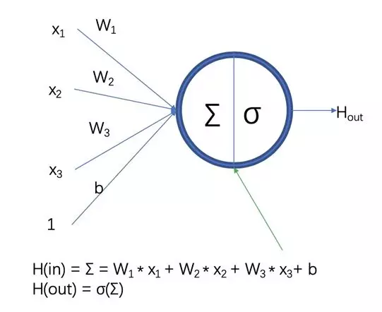
Figure 1. The Neural Cell
A neural network with only one hidden layer is called a shallow neural network. Consider the figure below for a visualization of what exactly a neural network is.
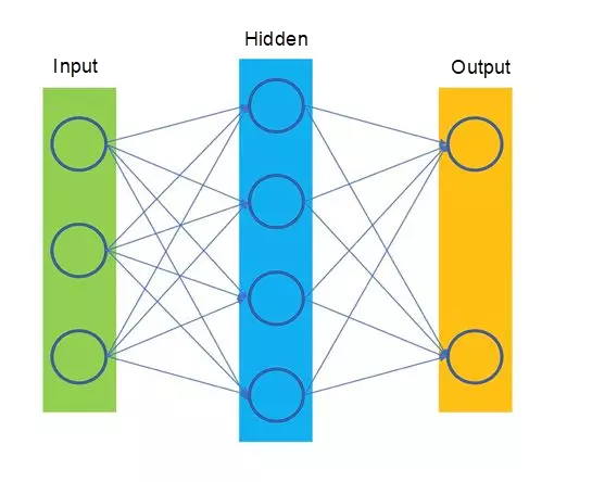
Figure 2. A Shallow Neural Network.
In contrast with a shallow neural network, a deep learning network has two, three, or more hidden layers, which are collectively known as a Multilayer Perceptron (MLP).
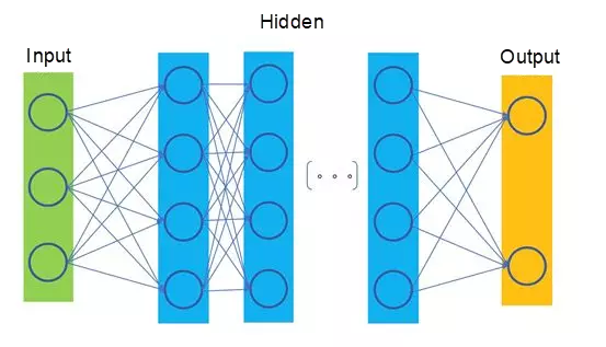
Figure 3. A Deep Learning Network
Generally speaking, a sufficiently wide network can fit any function. However, a multilayer perceptron can use fewer parameters to fit the function because neural cells on a multilayer perceptron can obtain more complex feature representations than those obtained by a shallow neural network.
The networks shown in Figure 2 and 3 are called fully connected networks. This is because neural cells at the hidden layers in these networks are related to the outputs of all neural cells at the upper layer. Corresponding to a fully connected network is a network on which neural cells are connected only to the outputs of some neural cells at the upper layer, for example, the convolutional neural network described below.
Neural cells on the convolutional neural network (CNN) are connected only to the outputs of some neural cells at the upper layer. Intuitively, this is because the synapses of human visual neural cells are only sensitive to local information, and not all global information has an equivalent effect on the same synapse.
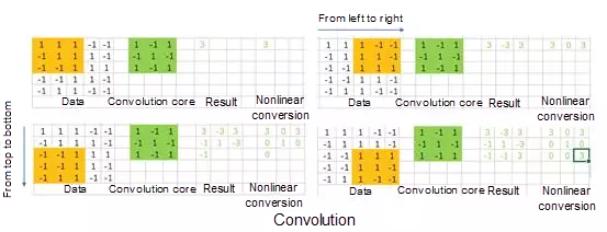
The same convolution core is multiplied with the inputs from left to right and from top to bottom to obtain the outputs of different strengths. Intuitively, the sensitivity of the convolution core to different data distributions of raw data is different. If the convolution core is construed as a certain pattern, a data distribution conforming to this pattern will produce a strong output, and a data distribution not conforming to this pattern will produce a weak output or even none output.

A convolution core is a pattern extractor, and multiple convolution cores are multiple pattern extractors. Using multiple feature extractors to extract and convert the features of raw data constitutes a layer of convolution.
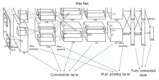
Due to the nature of GPU memory, the example above Alex Net uses two GPUs to splice the model. In essence, the convolution layer is used for feature extraction, the max pooling layer is for strong feature extraction and decrease parameters, and the full connection layer is for involving all advanced features in the final classification decision.
Where recurrent neural networks (RNN) are different to convolutional neural networks (CNN) is that they extract temporal features rather than spatial features as CNN do.

On the recurrent neural network (RNN), x1, x2, x3, and xt are inputs in different time sequences, whereas the three matrices V, U, and W are shared. Meanwhile, the RNN saves its own status. The status changes with the input. Different inputs or inputs at different times vary in their effect on the status. Generally speaking, the status determines the final output.
Intuitively, we can understand that the RNN is a neural network (action) that can simulate any function. Together, the action and the RNN's own historical memory turn the RNN into a Turing machine.
One major problem with recurrent neural networks (RNN), however, is that a nonlinear operation σ exists and each step is transmitted through the continuous multiplication operation. As a result, the long sequence history information cannot be well transmitted to the end. In this context, the model of long short-term memory (LSTM) emerges to solve this problem.
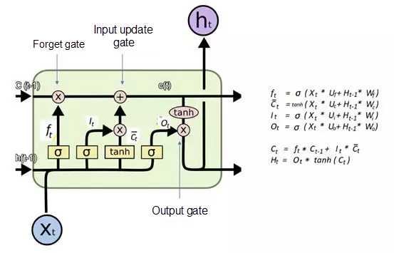
The LSTM cell contains the forget gate (dot product, which determines what needs to be removed from the status), input update gate (bitwise addition, which determines what needs to be added to the status), and output gate (dot product, which determines the status output). Although LSTM looks complex, in reality it is essentially a matrix operation.
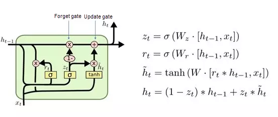
To simplify the operation, a gated recurrent units (GRU) variant of the LSTM is provided, as shown below:
Convolutional neural networks (CNN) are widely used in the computer recognition field for their powerful and generally accurate capability to capture local features, providing great help for researchers who analyze and utilize image data. Convolutional neural networks for text classification (TextCNN) was proposed by Yoon Kim during 2014 Conference on Empirical Methods on Natural Language Processing (EMNLP 2014) to apply the CNN to text classification tasks in natural language processing.
TextCNN uses one-dimensional convolution to obtain the feature representations of n-gram in a sentence. TextCNN is excellent in extracting superficial features of texts. It is widely used in the short text field, such as the search or dialog field. It is often the first choice for intent classification. In the long text field, TextCNN uses the filter window to extract features. Therefore, TextCNN has limited capabilities in long-distance modeling and is not sensitive to the word order.
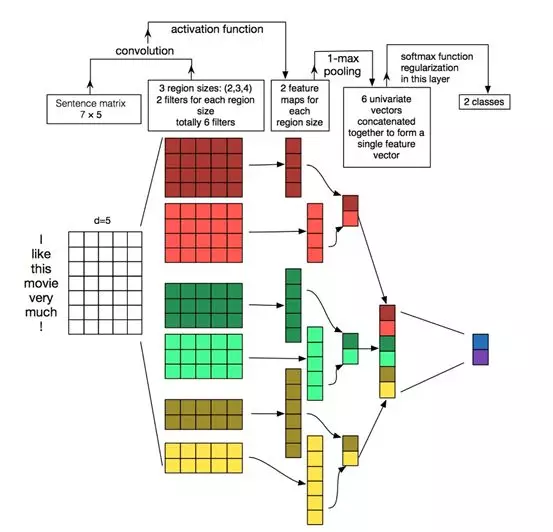
Now there's the convolution core (filter) and the N-Gram feature to talk about. Unlike the case for image convolution, convolution is performed only in one direction of the text sequence in text convolution. Convolution is performed on each possible window of a word in a sentence to produce the feature map.

Where,  . The max-pooling operation is performed on the feature map, and the maximum value max {c} is used as the feature extracted by the filter. You can capture the most important features by selecting the maximum value of each feature map.
Each filter convolution core generates a feature. A TextCNN network contains many convolution cores of different window sizes, such as the commonly used filter size ∈{3,4,5} and featuremaps = 100 for each filter.
Next, there's the enhanced sequential inference model (ESIM), which is a powerful model that is often used in short text matching tasks. It enhances long short-term memory (LSTM) mainly by outputting two input LSTM layers (encoding layers) into a new representation through the sequential inference interaction model.
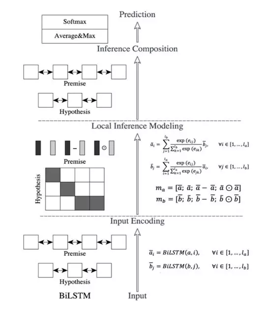
Image source: Enhanced Long Short-Term Memory (LSTM) for Natural Language Inference
As shown in the figure, the enhanced sequential inference model is on the left part of the figure. The overall network structure is clear. The entire path consists of three steps:
The embedding from language model (ELMo) solves the polysemy problem. For example, when you query what is the word vector of "Apple" and what context of "Apple" will be considered in ELMo, you should query what is the word vector of "Apple" in "Apple stock price". ELMo effectively captures the context by providing a dynamic representation that is of the word level and contains the context information. The proposal of ELMo has a good guiding and inspiration effect on Generative Pretained Transformer (GPT) and Bidirectional Encoder Representations from Transformers (BERT) that come later. A good word vector must have two characteristics:
Traditional Word2vec has only one fixed embedding expression for each word, and does not generate any embedding that carries the context information. Therefore, Word2vec cannot judge polysemous words based on the context. Each word in ELMo must be expressed through the multi-layer Long Short-Term Memory (LSTM) network in combination with the context. LSTM is created to capture context information. Therefore, ELMo can combine more contexts, and better handle the polysemy problem than Word2vec.
The network structure diagram of ELMo pre-training is similar to the traditional language model. It can be understood that the nonlinear layer in the middle is replaced by LSTM. The LSTM network is used to better extract the context information of each word in the current context, and meanwhile add the forward and backward context information.
Given a sequence containing N words  , the forward language model predicts the kth word
  based on the previous (k-1) words
  . At position k, each LSTM layer outputs the context-dependent vector expression
  , J = 1, 2 ,..., L. The output
  at the top LSTM layer uses cross entropy loss to predict the next position
  .
.

The backward language model reverses the sequence and uses subsequent words to predict previous words. Similar to the forward language model, for the given sequence  , the hidden layer output
  at layer j is obtained through the prediction of the deep LSTM network at layer L.

The two-way language model splices the forward language model and the backward language model together to construct the maximum logarithm likelihood of forward and backward joins.

Where,  is a parameter of the sequential word vector layer, and
  is a cross entropy layer parameter. Both parameters are shared in the training process.
The combination of the embedded language models uses the internal information of the multi-layer LSTM layer to compute the center word and uses the two-way language model at layer L to obtain (2L + 1) expression sets.
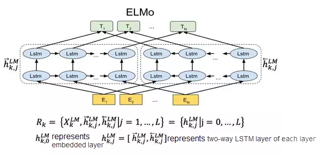
In downstream tasks, ELMo integrates the outputs of multiple layers into a vector, and adds the outputs of all LSTM layers to the normalized weight learned from Softmax, that is, s = Softmax (w). The detailed usage is as follows:
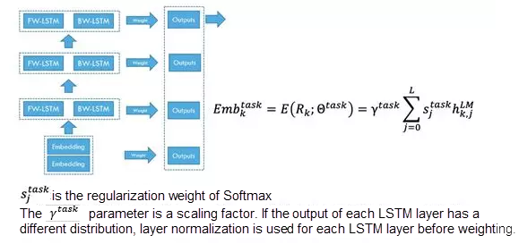
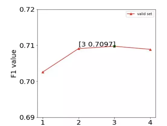
The higher-level LSTM vectors of biLMs capture the semantic information of words, whereas the lower-level LSTM vectors of biLMs capture the syntax information of words. The hierarchical effect of this depth model makes it possible to apply a set of word vectors to different tasks, because the amount of information required by each task is different. In addition, the number of LSTM layers should not be too large. A multi-layer LSTM network is difficult to train and suffers from an over-fitting problem. The following figure shows the experiment result of a multi-layer LSTM for text classification. As the number of LSTM layers increases, the model effect first increases and then decreases.
It is said that only one attention is required for improving the LSTM effect. But now, attention is all you need. The transformer solves the training problem of a deep network in the field of natural language processing.
Attention was previously used for many natural language processing tasks to locate key tokens or features. For example, an attention layer can be added at the end of text classification to improve performance. Transformer is originated from the Attention mechanism and completely abandons the traditional recurrent neural networks. Its network structure is completely based on the Attention mechanism. Transformer can be built by stacking transformer layers. In our experiment, a total of 12 layers of encoder-decoder, namely 6 layers of encoder and 6 layers of decoder, were built, and a record-high BLEU value was achieved in machine translation.
The following figure shows the entire flow. In this flow, it is assumed that the N value equals to 2 and the actual N value of Transformer is 6.
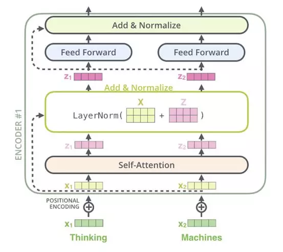
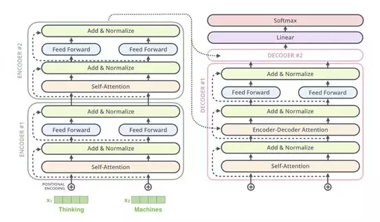
The structure of Transformer is easy to understand, but it contains many fragments, such as Multi-Head Attention, Feed Forward, Layer Norm, Positional Encoding, and so on.
Advantages of Transformer:
Comparison of the CNN, RNN, and Self-Attention:
Last, we now finally arrive at the Bidirectional Encoder Representations from Transformers (BERT), which we can define as a language model at the bottom layer in natural language processing. Through massive corpus pre-training, BERT can obtain the most comprehensive local and global feature representations of a sequence.
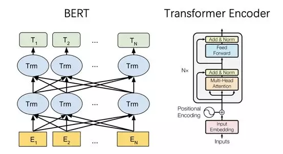
The following figure shows the network structure of BERT. The network structures of BERT and Transformer are identical. Assume that the dimension of the Embedding vector is that the input sequence contains n tokens, the input of a layer in the BERT model is a matrix, and its output is also a matrix. Therefore, N BERT layers can be easily connected in series. The large model of BERT uses a Transformer block with N = 24 layers.
1. Masked Language Model
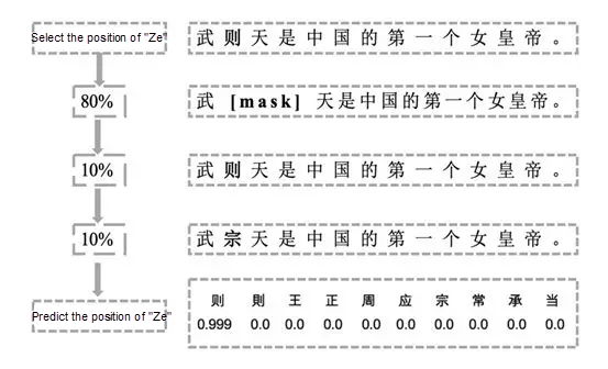
The masked language model (MLM) is used to train the deep two-way language to represent vectors. BERT uses a very direct way to mask some words in a sentence and let the encoder predict what these words are. The following figure shows the specific procedure. First, drop some words using a small probability mask. Then, use the language model to predict these words based on the context.
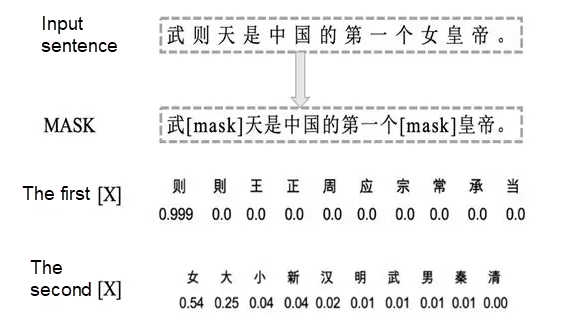
The specific training method of BERT is to randomly mask 15% of words as training samples.
Only 15% of words are masked due to the performance overhead. Anyway, training a two-way encoder is slower than training a one-way encoder. The 80% and 20% of words are selected because the mask is made during pre-training. When a specific task, such as a classification task, is fine-tuned, the input sequence is not masked, resulting in gap and inconsistent tasks. 10% of words are replaced by a random word and another 10% remain unchanged because the encoder does not know which words need to be predicted and which words are incorrect. Therefore, the encoder is forced to learn the representative vectors of each token to make a compromise.
2. Next Sentence Prediction
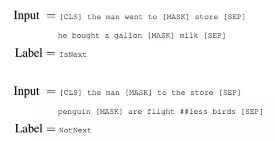
A binary classification model is pre-trained to learn the relationship between sentences. The method for predicting the next sentence is helpful for learning the relationship between sentences.
The detailed training method is as follows. The ratio of positive samples to negative samples is 1:1, and 50% of sentences are positive samples. That is, for given sentences A and B, B is the next sentence in the actual context of A. A sentence is selected randomly in the corpus and is used as B, that is, the negative sample. Two specific token [CLS] and [SEP] are used to concatenate two sentences. This task outputs a prediction at the [CLS] position.
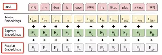
During pre-training, [CLS] does not participate in masking. Therefore, this position attends all positions of the entire sequence, and the output of the [CLS] position is sufficient to represent the information of the entire sentence, similar to a global feature. The embedding corresponding to the word token focuses more on the semantics, syntax, and context representation of the token, similar to a local feature.
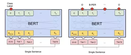
For different tasks, BERT uses different parts of output for prediction. The classification task uses the embedding at the [CLS] position, and the NER task uses the output embedding of each token.
The main contributions of BERT are as follows:
In the task of natural language understanding intent classification, we have practiced the above mainstream models, including XGBoost, TextCNN, LSTM, BERT, and ERNIE. The following is the early stage of model research. The BERT model shows great advantages in the comparative experiments on the selected test data.

At the same time, in the online deployment process, the BERT time consumption is tested, and the test results on the pressure test data are for reference. For our question and answer query:

In the image field, AlexNet opens the door of in-depth learning, and ResNet is a milestone of in-depth learning in the image field.
With the rise of Transformer and BERT, the network is also evolving to 12 or 24 layers, and SOTA is achieved. BERT has proved that in natural language processing, the effect of deep networks is better than that of shallow networks.
In the natural language field, Transformer opens the door of deep networks, and BERT becomes a milestone in natural language processing.
1 posts | 0 followers
Followqixiang.qx - February 6, 2020
dehong - July 8, 2020
Alibaba Clouder - July 22, 2020
Alibaba Clouder - March 2, 2018
Merchine Learning PAI - February 25, 2021
Alibaba Clouder - June 29, 2020
1 posts | 0 followers
Follow Platform For AI
A platform that provides enterprise-level data modeling services based on machine learning algorithms to quickly meet your needs for data-driven operations.
Learn More Black Friday Cloud Services Sale
Get started on cloud with $1. Start your cloud innovation journey here and now.
Learn More Epidemic Prediction Solution
This technology can be used to predict the spread of COVID-19 and help decision makers evaluate the impact of various prevention and control measures on the development of the epidemic.
Learn More