The previous blog post, Introduction to Machine Learning, presented the Machine Learning concept. Now, let’s discuss representative methods used in the technology. 
In most Machine Learning courses, regression algorithms are the first to be introduced for two reasons:
There are two regression algorithm subtypes: linear regression and logistic regression.
We have already touched on linear regression via the House Price Problem. Let’s figure out how to find the straight line that best fits all the data.
The "least squares" method is used to solve this problem. The thinking behind this method is: to find the line that best represents a set of data; and find
the line that most closely follows the observed data points in the data set. Not all of the data points lie exactly along a straight line, so the best fit line is
the one with the least deviation from those points. To minimize the deviation, find a straight line that minimizes the sum of the squares of all the
distances between the points and the line. The least squares method converts an optimization problem into an extreme function value problem. In
mathematics, we can find the extreme values of a function by looking at the point where the derivative is 0. However, this method is not suitable for
computers because they may fail to solve the problem or the computation may be too intensive.
In computer science, there is a specialized discipline called numerical computation. It strives to increase accuracy and efficiency when computers run
various computations. For example, the famous gradient descent method and Newton method are classic numerical computation algorithms. They are
also well-suited to find extreme values of functions. The gradient descent method is one of the simplest and most effective methods for solving regression
applied in other algorithms.
Logistic regression algorithms are similar to linear regression algorithms. However, the types of problems addressed by linear regression are different
from those addressed by logistic regression. Linear regression deals with numerical problems with final predictions being numbers, such as a house price.
Logistic regression, on the other hand, is used in classification algorithms. The predictions made out of logistic regression are discrete classes like logistic
regression is often used to determine a spam email or if a user will click on an advertisement.
In practice, logistic regression simply adds a Sigmoid function to the results computed by linear regression. This function converts the numerical result
into a probability between 0 and 1 (images of the Sigmoid function are not very intuitive, but you need to understand that larger values are closer to 1
and smaller values are closer to 0). Next, we make a prediction based on this probability. For example, if the probability is greater than 0.5, we can classify
an email as spam or judge a tumor to be malignant. For better understanding, refer to the logistic regression algorithm shown as a classification line in
the following figure.
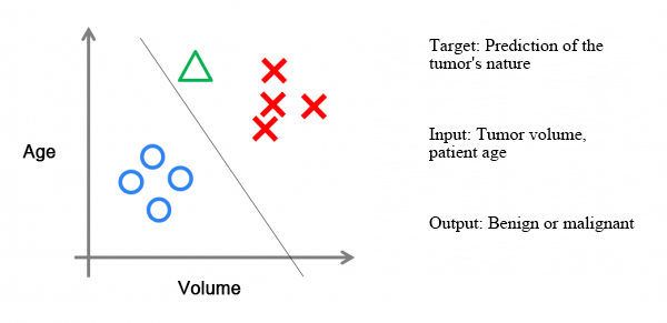
Assume there is a set of data on cancer patients. Some of these patients' tumors are benign (blue circles), while some are malignant (red Xs). The
tumors' red or blue markings are data "tags." Each data point includes two features: patient's age and tumor size. You can map these two features and
the data tags in two-dimensional space.
Now, there is a new data point (green triangle) to help determine if this tumor is malignant or benign. To do this, you can train a logistic regression
model based on the red and blue data points. This is the classification line shown in black. The green point is to the right of the classification line, so you
can determine that the tag should be red, indicating a malignant tumor.
The classification lines drawn by logistic regression algorithms are always linear (sometimes logistic regression uses non-linear lines, but these models
suffer from low efficiency when processing large volumes of data). Therefore, when a line dividing two classifications is not linear, logistic regression is
unable to express the situation adequately. Next, let's discuss the two most powerful and important algorithms used in ML. Both are used to find non-
linear classification lines.
Neural network algorithms (also called artificial neural networks or ANN) are used widely in deep learning, neural networks have returned. They are
one of the most powerful Machine Learning algorithms.
Neural networks originated from the study of brain mechanisms. Biologists used neural networks to simulate the brain. Then, Machine Learning
academics used neural networks to perform Machine Learning experiments and found that they performed quite well for visual and audio recognition.
The specific learning mechanisms of neural networks decompose and integrate data. In the famous Hubel-Wiesel experiment, researchers investigating
the visual analysis mechanisms of cats found this to be the mechanism at work.
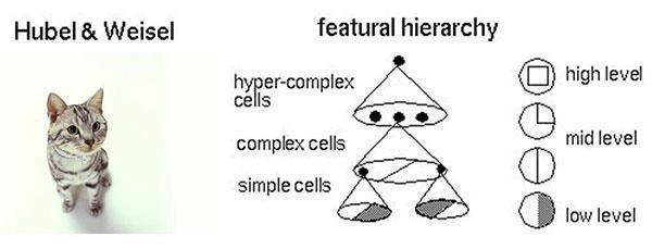
For instance, a square features four polylines and then enters the next layer of visual processing. Each of the four neurons is used to process one
complex image converts into data when entering neurons. After being processed by the neurons, it is integrated. Finally, the brain sees the resulting
Let's now look at the logical structure of a simple neural network. This network can be divided into input, hidden, and output layers. The input layer
receives signals; the hidden layer analyzes and processes data; and the final result is integrated into the output layer. In each layer, the circles represent
processing units. These can be thought of as simulated neurons. Several processing units combine to form a layer, and several layers form a network. The
result is a neural network.
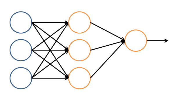
In a neural network, each processing unit is a logistic regression model that receives input from the upper layer and outputs prediction results to the
next layer. Through this process, neural networks can accomplish complex, non-linear classification.
The following figure demonstrates a famous application of neural networks in the image recognition field. The program is called, LeNet, and the neural
network is constructed with multiple hidden layers. LeNet can recognize numbers written in different ways to achieve a high degree of accuracy and
robustness.
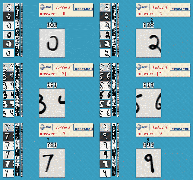
The square at the center shows the images put into the computer. At the top, the red number after "answer" is the computer's output. The three
columns on the left-hand side of the image show the output of the neural network's three hidden layers. As the layers become deeper, there is less detail,
like we see that , the basic processing in layer three has reached only linear detail.
In the 1990s, the development of neural networks encountered a bottleneck because even with BP algorithm acceleration. therefore, in the late
1990s, SVM algorithms replaced neural networks.
Support vector machine algorithms originated from the statistical learning field and came into their own as a classic algorithm in the ML field.
In a sense, SVM algorithms are enhancements of logistic regression algorithms. By providing logistic regression algorithms with stricter optimization
conditions, SVM algorithms draw better classification boundary lines than traditional logistic regression.
When combined with a Gaussian "core," SVM can express extremely complex classification borders to produce better classification results. The "core"
is a special function. The most typical feature of such a function is that it can map data from low-dimensional space to high-dimensional space.
&nbps;&nbps; Here is an example:
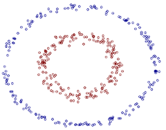
Now, the issue becomes how to draw a circular classification border in two-dimensional (2-D) space, which is difficult. However, use the "core” to
map the 2-D data to three-dimensional (3-D) space. Then, use a linear plane to achieve similar results. Hence, a non-linear classification border in 2-D
space is equivalent to a linear border in 3-D space. You can therefore use a simple line to divide data in 3-D space and achieve the effect of a non-linear
division in 2-D space. The following is a section of 3-D space.
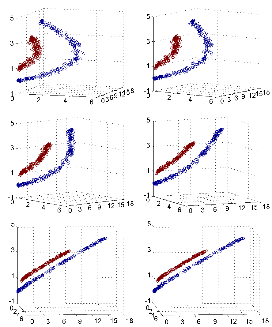
SVM algorithms are mathematical ML algorithms (comparatively, neural networks have a biological component). The core step of the algorithm offers
further proof that data mapped from low-dimensional space to high-dimensional space does not increase the complexity of the final computation.
Therefore, SVM algorithms help maintain computational efficiency and deliver improved classification results.
For all the previously mentioned algorithms, one prominent characteristic is that the training data contains tags and trained models can predict tags
for unknown data. In the following algorithms, the training data does not include tags, and the algorithms strive to infer these data tags through training.
These algorithms have a common name: unsupervised algorithms (algorithms that use tagged data are supervised algorithms). Typical unsupervised
algorithms are clustering algorithms. Returning to 2-D data, you can say that each data point has two features.
How can you use a clustering algorithm to mark them with various tags? Simply put, a clustering algorithm computes the distance between
groupings and based on these distances, divides data points into multiple groups. The most typical example of a clustering algorithm is the K-Means
algorithm.
A descending dimension algorithm is a type of unsupervised algorithm. It reduces data from a high-dimensional level to a low-dimensional level.
Dimensions represent the size of features that characterize the data. For instance, house price data may have four features: house length, width, area, and
number of rooms. Therefore, it is four-dimensional (4-D) data. The features of length and width overlap with the area feature because area = length x
compress 4-D data into 2-D data.
You can use mathematics to prove that an algorithm compresses the number of dimensions while retaining the maximum amount of information.
Thus, descending dimension algorithms are still advantageous.
They are primarily used to compress data and enhance the efficiency of other ML algorithms. Another advantage is visualization. For example, if you
compress five-dimensional (5-D) data into 2-D data, the data can be visualized on a 2-D plane. Principal Component Analysis (PCA) algorithms are the
most typical example of a descending dimension algorithm.
Recommendation algorithms are very popular in the ML industry and widely used by e-commerce companies, such as Amazon, Tmall, and Jingdong.
The primary characteristic of recommendation algorithms is that it automatically recommends things that most interest a user to increase purchase rates.
There are two main types of recommendation algorithms.
Algorithms that give recommendations based on item content.These algorithms recommend items to a user that are similar to their recent purchase. They require each item to have several tags in order to find
items similar to the user's purchased items. The advantage of these recommendations is their high degree of relevance.
They show the user recommendations based on items purchased by other users with the same interests. For example, if user A has purchased items B
and C and the algorithm discovers that user D has the same interests as user A, and has bought item E, it will recommend item E to user A.
Both types of recommendation algorithms have their respective advantages and disadvantages. In e-commerce applications, sellers use a mix of both
In addition to the algorithms previously mentioned, many others are used in Machine Learning, such as Gaussian discriminant, naive Bayes, and
decision tree algorithms. Howevjer, the six algorithms discussed previously are the most widely used, have the greatest impact, and are the most
representative types.
Here is a summary of the algorithms:
In addition to these algorithms, there are some algorithms whose names are often mentioned in the Machine Learning field. However, these are not
true Machine Learning algorithms. Instead, they originated from attempts to solve some sub-problems. Among these "sub-algorithms," the most
representative is the gradient descent method, mainly used in linear regression, logistic regression, neural networks, and recommendation algorithms;
Newton method, used in linear regression; BP algorithms, used in neural networks; and SMO algorithms, used in SVM.
In this blog post, we learned about algorithms that help implement ML functions. These include regression algorithms, neural networks, SVM,
clustering algorithms, descending dimension algorithms, and recommendation algorithms. In the next blog post, Machine Learning Applications, we look
at its applications in related fields, including big data, artificial intelligence, and deep learning.
"Massive sales… just for you!" - The Art of Personalized Marketing

2,593 posts | 793 followers
FollowAlibaba Clouder - July 17, 2020
Alibaba Clouder - July 17, 2019
Alibaba Clouder - December 26, 2016
Farah Abdou - November 27, 2024
Alibaba Clouder - December 30, 2020
Alibaba Clouder - March 11, 2021

2,593 posts | 793 followers
Follow AI Acceleration Solution
Accelerate AI-driven business and AI model training and inference with Alibaba Cloud GPU technology
Learn More Tongyi Qianwen (Qwen)
Top-performance foundation models from Alibaba Cloud
Learn More Alibaba Cloud for Generative AI
Accelerate innovation with generative AI to create new business success
Learn More AgentBay
Multimodal cloud-based operating environment and expert agent platform, supporting automation and remote control across browsers, desktops, mobile devices, and code.
Learn MoreMore Posts by Alibaba Clouder