Optimizing Complex Data Distribution in MaxCompute

For a long time, data distribution has been an issue in the field of Big Data processing. Unfortunately, the Big Data processing systems that are popular today do not satisfactorily solve the issue. In the all-new optimizer for Maxcompute2.0, we introduced complex data distribution. In this version we added new optimization measures like partition pruning, distribution pull up and push down, and distribution alignment. This article begins with the principle and history of data distribution, explaining our thoughts and solutions on the matter.

Understanding Data Distribution

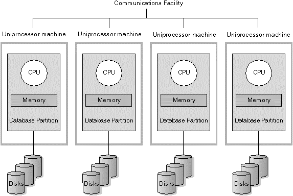
For many people, bringing up data distribution arouses thoughts of MPP DBMS. In fact, we often say that one only needs to think about data distribution when using MPP DBMS. First, let’s take a look at the categorization of databases:

Shared Everything: The difference between this type and the following two is that this one is typically not distributed.
Shared Disk: The database server is horizontally expandable and does not have storage of its own. It uses SAN or NAS technology to connect to the backend where it can horizontally expand across unified storage. The network connection on this layer as well as the expandability of the database server limit the Shared Disk. Oracle RAC and other commercial distributed databases belong to this category.
Shared Nothing: Unlike Shared Disk, this type of framework utilizes co-located database servers and storage on the same node. This means that physical nodes do not share anything, significantly decreasing network IO. MPP DBMS and Hadoop belong to this category.

Obviously, when deploying a Shared Nothing database, you need to carefully consider data distribution. You first need to know how to distribute data across different physical nodes (since this database doesn’t place data into unified storage unlike the Shared Disk system) to reduce the demands of future operations. For example, in Greenplum, one has to define a partition key when building a table, after which the system will distribute data according to key (hash). If we partition the two tables in a Join operation according to join key, then the Join operation will not require network IO. If one of the involved tables uses a different group of partition keys, then a re-partitioning operation may be necessary.

This is precisely why we need to understand the principle behind data distribution, as it can be critical to the application and system optimization. There is a significant amount of information available concerning data distribution on MPP DBMS. But why don’t these kinds of optimizations exist for data processing systems like Hadoop? Simply put, it’s because then we need stronger expandability (and support for unstructured data, but we won’t go into that).

The difference is that MPP and Hadoop don’t place data and computing on the same node. Even if we were to do so, it would limit the system expandability. Dynamic expandability especially suffers. Take into consideration a group of 50 currently operating Greenplum clusters. It would be nearly impossible to quickly add, for example, two new nodes and still maintain efficient operation. Hadoop is very good at this, the main solution being:

Separation of storage and computing
Centralized settings support highly efficient peer to peer reading and writing (HDFS)

This is why, when you create a table in Hive, you don't need to define a partition key like in Greenplum. Also, this explains why Join operations are less efficient in Hive than they are in Greenplum.

The Goal of Data Distribution Optimization

As described above, Big Data distribution systems often trend toward random distribution regarding storage, increasing expandability at the cost of performance. However, re-examining this trade-off, using random distribution in storage doesn’t mean that we can't take advantage of data distribution optimized searches. The goal of distribution optimization is to utilize already existing distribution and satisfy future demands to the furthest extent possible. This kind of optimization includes:

Partition Trimming
Using the characteristics of data distribution, we can use partition trimming to reduce data reads. For example, we can apply partition trimming to hash distribution for point queries, and range distribution for interval queries.
Elimination Redistribution
If the current distribution meets the requirements of future algorithms, we can eliminate extra redistribution operations. It is common knowledge that redistribution (called shuffle in Hadoop) is the primary resource consumer in distribution algorithms.
Avoiding Data Skew
We can use better data distribution algorithms to avoid data skew. For example, if we have some frequently repeating values (end-biased) in a data cluster, we can use range distribution rather than hash distribution. This will effectively help you in avoiding the performance loss caused by data skew.

Types of Data Distribution

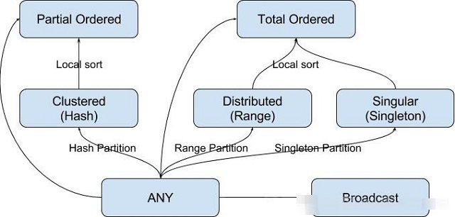
The following are examples of data distribution types and their meanings:

Type	Meaning	Required variable	Optional variable	Example
ANY	Any distribution	-	-	ANY
HASH	Hash distribution	Keys	numBuckets	HASH(c1)[100]
RANGE	Range distribution	Keys	Boundaries	RNG(c1){(100, 200], (200, 300]}
BROADCAST	Broadcast distribution	-	-	BROADCAST
SINGLETON	Single node distribution	-	-	SINGLETON

Data Conversion Relationship

Implementation

While adhering to Volcano optimizer syntax, we can turn distribution properties into a kind of physical property called distribution. Like other properties, it has ‘required property’ and ‘delivered property’ pairs. For example, for sorted merge join, it will apply a Partial Ordered required property to all input. At the same time, it will deliver a Partial Ordered property which gives following operations a chance to use this property and avoid a round of redistribution.

Consider the below query:

SELECT uid, count(*) FROM (
  SELECT uid FROM user JOIN line ON user.uid = line.uid
) GROUP BY uid

At this point, if Join becomes a Sorted Merge Join, it may deliver a Hash[uid] property, which is required by Aggregate, then we can skip an unnecessary round of redistribution.

If we want to apply a similar optimization, then we need to take into consideration the below issues:

Characteristics of aggregated distribution
(Local relational algebraic compilation) select a suitable distribution property
(Total cost calculation) avoid using the wrong distribution property

Characteristics of Aggregated Distribution

There are three ways to generate data distribution:

User defined: Just like MPP, we can introduce a partition key to DDL, allowing the user to specify the data distribution. Of course, unlike MMP, this kind of distribution only requires an index structure for a distributed file system and cannot connect physical nodes.
SQL logic: SQL logic could generate data distribution when being run. For example, a ‘distribute by’ statement declares that SQL logic would distribute data upon running.
Secondary application of algorithms: Each distribution algorithm could create a distribution upon running. For example, sorted merge join can ensure that its output data meets the ordering and hash distribution requirements of join keys.

Several algorithms require a special data distribution:

Aggregate: Sorted Aggregate requires grouping key and Hash distribution.
Join: Sorted Merge Join and Hash Join both require inputting the same Hash Distribution and join key.
Sort: ‘Order by’ requires Range distribution on sort key or Singleton distribution.

Choosing the Appropriate Distribution Property

Even if we have a series of required and delivered distribution properties, it’s still not easy to determine the kind of distribution needed for each operation. Unlike ordering properties (only includes row sequences and ascending or descending order properties), distribution properties vary significantly. The reason for this variance is:

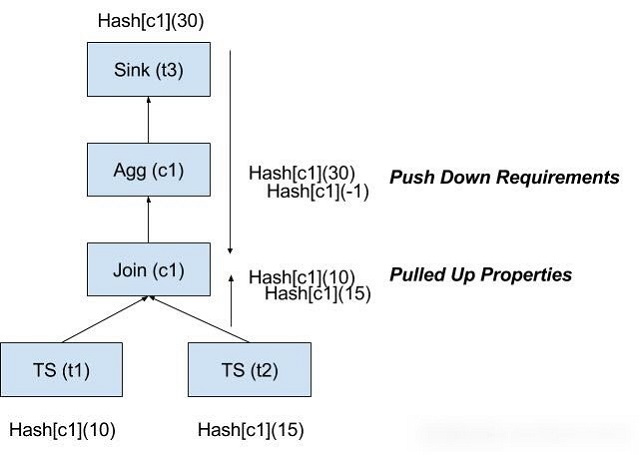
To provide different options to satisfy distribution requirements. For example, the aggregate group by a, b, c carries a Partial Ordered requirement for input data. Its ordering requirements are that a, b, and c be ordered. However, Hash (a), Hash (b), Hash (a, b), Hash (a, b, c), or RNG(a) could all satisfy the distribution requirements.
One can use a variety of options to achieve distribution. For example, in the join operation, join a and b on a.id = b.id, if a is subject to Hashid, and b is subject to Hashid, then for Sorted Merge Join, you can choose to require Hashid, Hashid, or any Hash(id) really.

The complexity leaves more room for finding the most optimal method. In reality, finding the most optimal method is a question of the NPC of the number of relational algebra numbers. To reduce the space that under the search, we use a heuristic branch selection algorithm. When compiling a relational algebra, we not only need to satisfy the needs of subsequent operations, we also need to think about the probability that prior operations will be able to produce satisfactory distribution. To realize the latter, one can use a module called Pulled Up Property.

Pulled Up Property guesses and screens for possible preliminary delivered properties that we can use to narrow down searches during compilation. Consider the query in the above image. When compiling Join, because Sink requires a push-down operation, it needs to provide a Hash[c1](30). Pulled Up Property then guesses that prior operations will possibly provide Hash[c1](10) and Hash[c1](15). Considering that Join will directly require Hash[c1](30), it then reduces the Hash[c1](10) and Hash[c1](15) branches.

Avoiding Improper Distribution Properties

Data skew occurs when we store the majority of data on a minority of nodes during data distribution. It reduces the entire algorithm to single machine operation. Under Partitioning occurs when we specify very few nodes during distribution. It means that one cannot efficiently utilize the distribution resources. Of course, we hope to avoid these two situations.

These avoid these situations we need better statistical information. When an optimization plan encounters Data Skew or Under Partitioning, we need to apply the proper penalty to its cost estimation, decreasing its selection likelihood in the future. We define “good” distribution as one where the amount of data processed by each node falls within a certain pre-defined range. If data processing for a single node is lower or higher than this range, then it should penalize the distribution. Factors that go into estimating this data volume include:

Row count (number of input records)
Top values (data with the most repetitions)
Histogram

Summary

In this article, we have gone over the significance of data distribution optimization and explained how to optimize data distribution in MaxCompute. We have already embodied these optimizations in the latest release of MaxCompute.

Looking at our tests, the effects of the optimization are undeniable. After applying to appropriate partitioning to TPC-H, we see that overall performance increasing by order of 20%. Even if do not partition the data on the table, partition optimization while running transparently to the user is very effective. When running in an online environment, 14% of queries were able to skip a step of redistribution because of these optimizations.

Community

Optimizing Complex Data Distribution in MaxCompute

Understanding Data Distribution

The Goal of Data Distribution Optimization

Types of Data Distribution

Data Conversion Relationship

Implementation

Characteristics of Aggregated Distribution

Choosing the Appropriate Distribution Property

Avoiding Improper Distribution Properties

Summary

Read previous post:

Read next post:

Alibaba Clouder

You may also like

Comments

Raja_KT March 16, 2019 at 3:45 am

Alibaba Clouder

Related Products

Big Data Consulting for Data Technology Solution

MaxCompute

Big Data Consulting Services for Retail Solution

Data Lake Storage Solution