
The foremost goal of this technology is to correctly and efficiently respond to user demand. In this article, we will take a look at the basic technical architecture of keyword spotting technology, along with the newest research results given during Interspeech 2017,held on August 20-24 in Stockholm, Sweden, and attended by participants from renowned companies, universities, and research institutes, as well as a high-profile team from Alibaba group.
This article covers the topic shared in the second session, that is, keyword spotting technology.
Keyword spotting means that when a user speaks certain voice demands, the device switches from sleep mode to working mode, and responds as requested.
The above four diagrams depict the process of keyword spotting from sleep mode to working mode. First, the device turns on, loads the resources, and enters into sleep mode. When a user speaks out certain keywords, they are spotted, and the device switches to working mode, waiting for further demand from the user. From this process, we can learn that the user can operate the device completely just by using voice, without the need of hands. At the same timeemploying the keyword spotting mechanism saves a lot of energy as the device is not in working mode constantly.
Keyword spotting technology has a wide scope of application, such as robots, mobile phones, wearables, smart homes, and vehicle mounted electronics. Many devices with a voice recognition function can use keyword spotting as the start of human-machine interactions. The products shown in below charts carry the keyword spotting technology, and there are many such products. As mentioned above, for the device to spot the keyword, a user needs to speak out certain keywords, which are different for different products. Keywords are chosen according to certain rules, and usually include three to four syllables. Keywords with more unique syllables are deemed better.
There are four evaluation indicators for keyword spotting.
1) Recall rate, which means correct spotting times as percentage of total times that the keyword should be spotted. Higher recall rate means better performance.
2) False alarm rate, which means the probability of keyword being spotted that should not be spotted. Lower false alarm rate means better performance.
3) Real time factor- from a user experience perspective, real time factor means reaction speed of the device. For keyword spotting, it is demanding in terms of reaction speed.
4) Power consumption- As most devices are either rechargeable or powered by batteries, only low power consumption will guarantee long battery endurance.
Keyword spotting could be considered as a small-footprint keyword search task. It features limited computing and storage resources, so its system frame is somewhat different from keyword search. Currently there are two common system frameworks:
1) Keyword/filler system based on HMM
For this kind of system, decoding module is veryimportant. The module is similar with the decoder in voice recognition, obtaining the optimal path using Viterbi algorithm. The difference lies in the construction of decoding network. The decoding network in keyword spotting task also includes paths of keywords and filler words. All words are included in the path of filler except for keywords, which is different from voice recognition task where each word has its corresponding path. Such networks can decode the keyword in a well-directed manner, leading to smaller decoding network, relatively less alternative paths, and significantly increased decoding speed. After the keyword paths are found in decoding results, further choice and judgment can be made on keyword spotting.
2) End-to-end system
In this system, the input voice is directly translated into output keyword. This kind of system includes three steps. The first step is feature extraction. The second step is neural networks, which includes input voice features and output posterior probability of each keyword as well as other words. In this step, the posterior value is output in frames, so the third step is required to smooth the posterior value with a certain window length. If the smoothened posterior value exceeds a certain threshold, the keyword is regarded as spotted.
2.1 Paper 1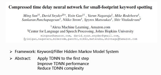
The first paper comes from Amazon, which adopts the first of its kind system in its architecture as introduced above. The focus of this article is the use of TDNN model as the acoustic model in the first decoding module. TDNN stands for Time Delay Neural Network as shown in the title of the paper. Meanwhile, TDNN computation is reduced using optimization is made to reduce TDNN computation, thereby meeting the real-time factor requirement.
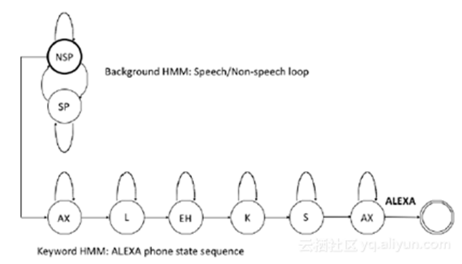
The above chart represents the decoding network of this system. The path below is the path of keyword Alexa and the path above is the path of filler, in which NSP represents the non-voice filler and SP means voice filler. Each circle in the chart stands for an HMM model. In the modelling module, phones are modelled using three-state HMM for keyword, while single-state HMM is used in modelling for the filler part. The TDNN mentioned above means modelling HMM emission probability using TDNN.
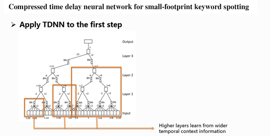
The structure of the TDNN used in this paper is illustrated in the above chart. TDNN learning needs the information kept from the former and latter frames. This chart represents the network structure of the frame at time t in time dimension. In the above chart, the orange frame means deeper layers can learn wider contextual information. For the modelling of this frame, input features of 30 frames from t-20 to t+10 are used, and more frames can be used through adjustment. Such long-term information learning can be impossible for DNN. So, the major advantage of TDNN is its capability to learn and handle longer contextual information.
To achieve better results in TDNN, this paper adopts two methods:
1) Transfer learning: Transfer learning is a widely-used method in machine learning. The core is to transfer the knowledge gained from a related task to the current task. In this task, a network for LVCSR tasks is trained first, and the LVCSR network parameter is taken as the initial value of network hidden layer parameter in the keyword spotting task, in order to start the training. This enables a better initialization for keyword spotting task network, and is helpful for final convergence to a better local optimal solution.
2) Multi-task: The multi-task learning using shared hidden layer structure. In this paper, there are two tasks, learning keyword spotting task as well as learning LVCSR. The two tasks share the input layer and most hidden layers. In the training, the object function is the weighted average of the two tasks, and the weightings can be adjusted. In the final use of this network, the node only related to LVCSR is carved out, so using it is the same as the ordinary model.
To meet the actual needs, this paper adopts two methods to reduce the amount of TDDN computation.
1) Sub-sampling: The original TDNN is a fully-connected network. But actually, the contextual information included in the neighboring time slot are in large part overlapping, so sampling method can be adopted to reserve only part of the connections, achieving similar effect as the original model, and significantly reduce the amount of model computation.
2) SVD (Singular-value Decomposition): It is used to transform a parameter matrix into the multiplication of two matrices. After the decomposition, the singular value would be sorted from the largest to the smallest. In most cases, the sum of the first 10% or even 1% singular value would dominate over 99% of the total singular value. So retaining only part of the singular value to optimize the computation amount will not cause function loss to the model if the retained value is reasonably chosen. Such structural adjustment can make the model structure even more reasonable and achieve better convergence point.
The experiment keyword is Alexa, and the data for training and testing is the far-field data fetched in different conditions in the room. The specific data volume is not provided, but the paper talks about sufficient training, developing and testing data.
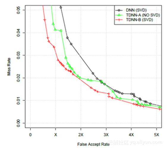
The above chart is the result of the experiment, with horizontal axis being the false-alarming rate, and vertical axis being the value of 1 minus recall rate. The curve above is called ROC curve, and lower curve means better performance. The comparison baseline is a DNN after SVD, as shown in the black line in the chart. Comparing the green line (no SVD) and red line (after SVD), which are the result of TDNN, we could conclude that TDNN is better than DNN, and SVD provides even further performance improvement for TDNN. From the result of AUC (area under curve), TDNN's performance is 19.7% higher than DNN, while the performance after SVD is 37.6% higher than DNN.
2.2 Paper 2 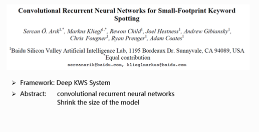
The second paper comes from Baidu, which adopts the second type of system or an end-to-end model, as introduced above. The most important part of this type of system is a neural network. This paper adopts a network structure called CRNN, and explores different model structures and parameters in order to simplify the model and achieve better performance. CRNN means combining CNN and RNN into one network, as CNN has the advantage of mining local information, while RNN is good at learning long time contextual information, and the two models can complement each other. Previously, Baidu used this model for LVCSR tasks, specifically CRNN plus CTC model, and achieved good result, so Baidu introduces it into the keyword spotting task. But currently CTC performs better for tasks with larger models and datasets, so cross entropy is still used as the object function in this paper. The adopted model network structure is illustrated as follows.
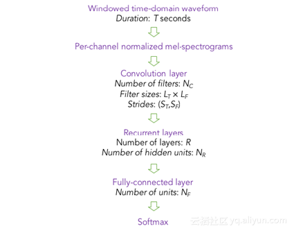
In the chart, the input is in the top part while the output is in the bottom. The input is voice with PCEN feature as a layer added into the network, and this feature has a good anti-noise ability. The following hidden layers include CNN, BiRNN, and DNN. The output layer includes 2 nodes, representing keywords and other words. In this structure, many manually adjusted parameters are included. For selecting RNN node structure, a comparison between many groups of parameter results and RNN nodes adopting LSTM and GRU are provided.
The experiment keyword is "talktype", and the training and testing data comes from over five thousand speakers, with no specific data given. In this paper, detailed experiments are conducted and useful conclusions are reached for reference in this paper. In the experiment analyzing the effect of data size on performance, positive and negative samples are added to improve the model performance. The experiment shows that positive samples can be beneficial for the model, and the model performance cannot be further improved if there are too many added samples. On the other hand, the addition of negative samples helps the model improve to an even greater extent. In the experiment testing far-field robustness, it is concluded that the training data should be selected carefully to reflect the actual application scenario. Another experiment compares CRNN and CNN. When signal-noise ratio is low, CRNN is better than CNN. But as the signal-noise ratio becomes larger, the performance gap between CRNN and CNN would be quite small. We can conclude that RNN is helpful in the case of low signal-noise ratio, or big noise. In the last part of the paper, a comprehensive result is achieved as follows:
In the condition of 0.5 FA/hour, when the signal-noise ratio is 5dB, 10dB and 20dB, the accuracy rate would be 97.71%, 98.71%, and 99.3% respectively.
2.3 Paper 3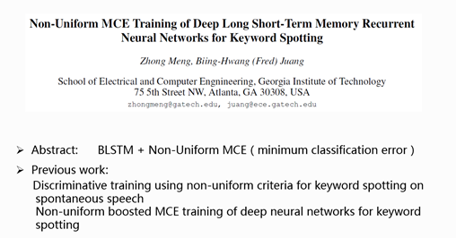
The third paper comes from Georgia Institute of Technology. This article targets keyword spotting, as keyword spotting can be thought of as a small-footprint, simplified keyword spotting. This article is useful in keyword spotting task for reference. Without any resource limit, the decoding network adopted in the article is the complete LVCSR decoding network. The major work is the adoption of BLSTM modelling structure for the improvement of decoding model, and the non-uniform MCE, a set of discriminative training criteria for model training. BLSTM model is advantageous in learning long time contextual information. MCE (Minimum Classification Error), delegating a set of discriminative training criteria. The discriminative training criteria are helpful for improving the discriminating capability of similar pronunciation. The use of non-uniform MCE comes from a problem that the author found in the system. Actually, the problem also exists in the first type of keyword spotting system. In this system, the acoustic model training used in the decoding module targets all words, which is different from the keyword spotting system, as the keyword spotting system cares more on keyword parameter indicators. So, the authors put up with non-uniform criteria, which enables the model focus more on keyword training.
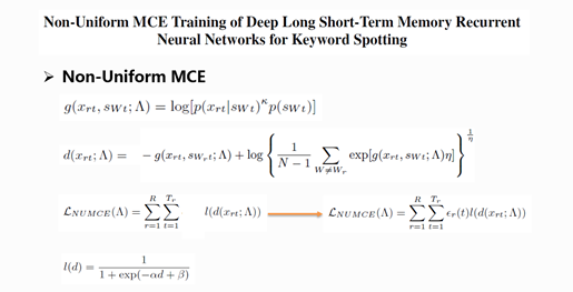
The first formula is frame level discriminative function and the second formula is the measure formula for misclassification. The third formula is the object function required by our neural network training, in which l function is a sigmoid function with parameters that are the measure of misclassification. The authors put up with non-uniform MCE, which adds the cost function ϵ_r (t) to the object function and gets the formula behind the arrow. By adding the cost function, the object function could render different punishment values on different kinds of errors, and effectively control the discriminative treatment among keyword misclassification errors and general classification errors. In actual use, the cost function would be iterated to reduce its effect by constantly multiplying coefficient 1, just like AdaBoost method. In addition, during the training process, the authors manually increase the likelihood value for the words with high phone error rate, and further improve the system. This is called BMCE.
The experiment is conducted on the switchboard for 300 hours, and the keyword in the task is about credit card use. FOM is adopted as performance indicators for different models: figure-of-merit, higher FOM means better performance. The experiment compares the DNN model and BLSTM model. The result is shown in the table below:
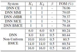
Performance comparison is shown in the above chart with different training criteria adopted on the DNN model. CE, short for cross entropy, is a generative training criterion, while the MMI, SMBR, MCE and BMCE are discriminative criteria. These discriminative criteria performs better than CE, and the non-uniform BMCE put up by the authors can further improve the performance. The optimal result has a 3.18% improvement as compared to CE criteria.
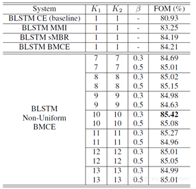
The performances with different training criteria adopted in the BLSTM model are shown in the above chart. As can be seen, this group of result is better than DNN. Using BLSTM, the training criteria put up by the authors are 5.55% better than the baseline.
Among the papers of Interspeech 2017, the keyword spotting technology papers mostly come from the actual products from renowned companies. The investigations conducted in these papers are helpful for the understanding of actual product performance and technical details, and good for reference. We hope this article helps you improve your understanding of keyword spotting technologies.
[1] Sun M, Snyder D, Gao Y, et al. Compressed Time Delay Neural Network for Small-Footprint Keyword Spotting[C]// INTERSPEECH. 2017:3607-3611.
[2] Arık S Ö, Kliegl M, Child R, et al. Convolutional Recurrent Neural Networks for Small-Footprint Keyword Spotting[C]// INTERSPEECH. 2017:1606-1610.
[3] Zhong M, Juang B H. Non-Uniform MCE Training of Deep Long Short-Term Memory Recurrent Neural Networks for Keyword Spotting[C]// INTERSPEECH. 2017:3547-3551.
[4] Weng C, Juang B H. Discriminative Training Using Non-Uniform Criteria for Keyword Spotting on Spontaneous Speech[J]. IEEE/ACM Transactions on Audio Speech & Language Processing, 2015, 23(2):300-312.
[5] Zhong M, Juang B H. Non-Uniform Boosted MCE Training of Deep Neural Networks for Keyword Spotting[C]// INTERSPEECH. 2016:770-774.
PhotoSharing Part I: Setting up the Photo Sharing Android Application

2,593 posts | 793 followers
FollowAlibaba Clouder - January 24, 2018
Alibaba Clouder - February 6, 2018
Alibaba Clouder - January 23, 2018
Alibaba Clouder - February 1, 2018
ApsaraDB - February 13, 2021
Alibaba Cloud Community - November 26, 2024

2,593 posts | 793 followers
Follow Intelligent Speech Interaction
Intelligent Speech Interaction is developed based on state-of-the-art technologies such as speech recognition, speech synthesis, and natural language understanding.
Learn MoreMore Posts by Alibaba Clouder