PolarDB for PostgreSQL supports the partition-wise join feature. When you join two partitioned tables on their partition keys, the default query planner joins all partitions against each other — including combinations whose key ranges never overlap. These mismatched pairs always return empty results and waste execution resources. Partition-wise join eliminates these invalid cross-partition joins by restructuring the plan so that only partitions with matching key ranges are joined. This reduces the amount of data scanned and significantly improves join query performance.
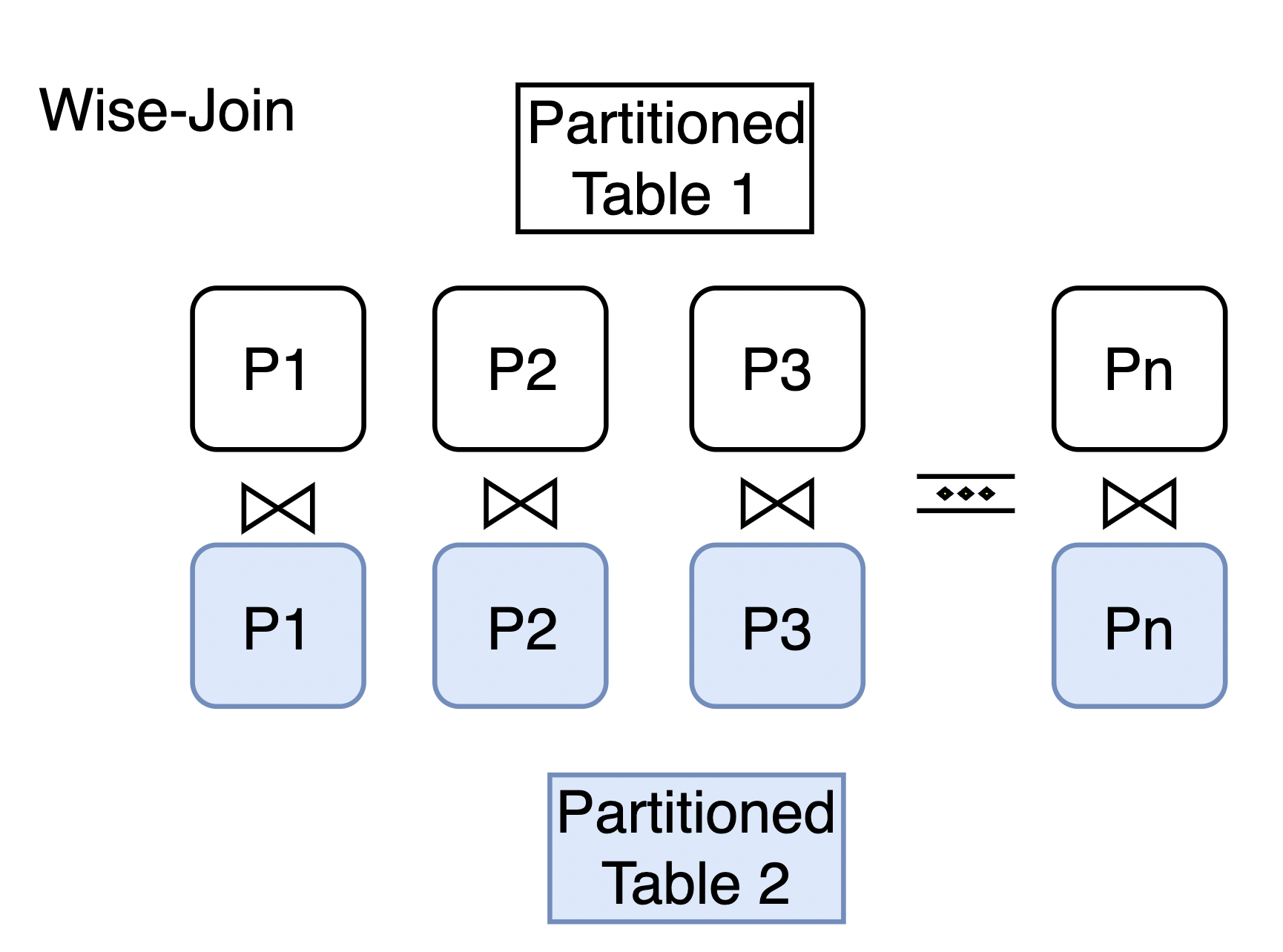
How it works
Without partition-wise join, the planner treats each table as a whole and produces a single join across all partition combinations. For example, joining sales_y2023q1 against measurement_y2023q3 always returns empty results, because the partition key ranges (2023-01-01 to 2023-04-01 vs. 2023-07-01 to 2023-10-01) never overlap.
With partition-wise join enabled, the planner recognizes that only partitions with matching key ranges can produce results. It decomposes the join into independent partition-pair joins, skipping all cross-partition combinations entirely.
Enable partition-wise join
Run the following statement to enable partition-wise join for the current session:
SET enable_partitionwise_join TO on;Example
The following example shows how partition-wise join changes the query plan for a join between two range-partitioned tables.
Set up the example tables
Create the measurement and sales tables, each partitioned by date range into four quarterly partitions covering 2023.
CREATE TABLE measurement(
    city_id         int not null,
    logdate         date not null,
    peaktemp        int,
    unitsales       int
) PARTITION BY RANGE (logdate);
CREATE TABLE measurement_y2023q1 PARTITION OF measurement
    FOR VALUES FROM ('2023-01-01') TO ('2023-04-01');
CREATE TABLE measurement_y2023q2 PARTITION OF measurement
    FOR VALUES FROM ('2023-04-01') TO ('2023-07-01');
CREATE TABLE measurement_y2023q3 PARTITION OF measurement
    FOR VALUES FROM ('2023-07-01') TO ('2023-10-01');
CREATE TABLE measurement_y2023q4 PARTITION OF measurement
    FOR VALUES FROM ('2023-10-01') TO ('2024-04-01');

CREATE TABLE sales (
    dept_no     integer,
    part_no     varchar(2),
    country     varchar(20),
    date        date,
    amount      decimal
) PARTITION BY RANGE (date);
CREATE TABLE sales_y2023q1 PARTITION OF sales
    FOR VALUES FROM ('2023-01-01') TO ('2023-04-01');
CREATE TABLE sales_y2023q2 PARTITION OF sales
    FOR VALUES FROM ('2023-04-01') TO ('2023-07-01');
CREATE TABLE sales_y2023q3 PARTITION OF sales
    FOR VALUES FROM ('2023-07-01') TO ('2023-10-01');
CREATE TABLE sales_y2023q4 PARTITION OF sales
    FOR VALUES FROM ('2023-10-01') TO ('2024-04-01');
Both tables have four partitions — one per quarter of 2023 — partitioned on their respective date columns (logdate for measurement, date for sales).
Compare query plans
Run the following join query and inspect the query plan:
EXPLAIN SELECT a.* FROM sales a JOIN measurement b ON a.date = b.logdate WHERE b.unitsales > 10;Without partition-wise join (default)
                                        QUERY PLAN
--------------------------------------------------------------------------------------------------
 Aggregate  (cost=871.75..871.76 rows=1 width=8)
   ->  Merge Join  (cost=448.58..812.79 rows=23587 width=32)
         Merge Cond: (a.date = b.logdate)
         ->  Sort  (cost=185.83..191.03 rows=2080 width=40)
               Sort Key: a.date
               ->  Append  (cost=0.00..71.20 rows=2080 width=40)
                     ->  Seq Scan on sales_y2023q1 a  (cost=0.00..15.20 rows=520 width=40)
                     ->  Seq Scan on sales_y2023q2 a_1  (cost=0.00..15.20 rows=520 width=40)
                     ->  Seq Scan on sales_y2023q3 a_2  (cost=0.00..15.20 rows=520 width=40)
                     ->  Seq Scan on sales_y2023q4 a_3  (cost=0.00..15.20 rows=520 width=40)
         ->  Sort  (cost=262.75..268.42 rows=2268 width=8)
               Sort Key: b.logdate
               ->  Append  (cost=0.00..136.34 rows=2268 width=8)
                     ->  Seq Scan on measurement_y2023q1 b  (cost=0.00..31.25 rows=567 width=8)
                           Filter: (unitsales > 10)
                     ->  Seq Scan on measurement_y2023q2 b_1  (cost=0.00..31.25 rows=567 width=8)
                           Filter: (unitsales > 10)
                     ->  Seq Scan on measurement_y2023q3 b_2  (cost=0.00..31.25 rows=567 width=8)
                           Filter: (unitsales > 10)
                     ->  Seq Scan on measurement_y2023q4 b_3  (cost=0.00..31.25 rows=567 width=8)
                           Filter: (unitsales > 10)
(21 rows)
The planner performs a single merge join across all data from both tables. This generates cross-partition joins that always return empty results — for example, sales_y2023q1 joined against measurement_y2023q3, where the key ranges (2023-01-01 to 2023-04-01 vs. 2023-07-01 to 2023-10-01) never overlap.
With partition-wise join enabled
SET enable_partitionwise_join TO on; QUERY PLAN
----------------------------------------------------------------------------------------
Append (cost=21.70..453.33 rows=5896 width=128)
-> Hash Join (cost=21.70..105.96 rows=1474 width=128)
Hash Cond: (b.logdate = a.date)
-> Seq Scan on measurement_y2023q1 b (cost=0.00..31.25 rows=567 width=8)
Filter: (unitsales > 10)
-> Hash (cost=15.20..15.20 rows=520 width=128)
-> Seq Scan on sales_y2023q1 a (cost=0.00..15.20 rows=520 width=128)
-> Hash Join (cost=21.70..105.96 rows=1474 width=128)
Hash Cond: (b_1.logdate = a_1.date)
-> Seq Scan on measurement_y2023q2 b_1 (cost=0.00..31.25 rows=567 width=8)
Filter: (unitsales > 10)
-> Hash (cost=15.20..15.20 rows=520 width=128)
-> Seq Scan on sales_y2023q2 a_1 (cost=0.00..15.20 rows=520 width=128)
-> Hash Join (cost=21.70..105.96 rows=1474 width=128)
Hash Cond: (b_2.logdate = a_2.date)
-> Seq Scan on measurement_y2023q3 b_2 (cost=0.00..31.25 rows=567 width=8)
Filter: (unitsales > 10)
-> Hash (cost=15.20..15.20 rows=520 width=128)
-> Seq Scan on sales_y2023q3 a_2 (cost=0.00..15.20 rows=520 width=128)
-> Hash Join (cost=21.70..105.96 rows=1474 width=128)
Hash Cond: (b_3.logdate = a_3.date)
-> Seq Scan on measurement_y2023q4 b_3 (cost=0.00..31.25 rows=567 width=8)
Filter: (unitsales > 10)
-> Hash (cost=15.20..15.20 rows=520 width=128)
-> Seq Scan on sales_y2023q4 a_3 (cost=0.00..15.20 rows=520 width=128)
(25 rows)The planner now joins each quarter's partition pair independently: sales_y2023q1 with measurement_y2023q1, sales_y2023q2 with measurement_y2023q2, and so on. All cross-partition joins are eliminated, reducing the total amount of data scanned and significantly improving join query performance.