A scatter chart is a component for visualizing data distribution. It is commonly used in regression analysis to display the distribution of data points on a Cartesian plane. By plotting the coordinates of each data point, scatter charts help identify correlations, trends, and outliers between variables.
Configure the component
Method 1: Use the GUI
On the Designer workflow page, add the Scatter Chart component. Then, configure its parameters in the pane on the right.
|
Parameter |
Description |
|
Feature columns |
Select the columns that represent the features of the training data. |
|
Classification label column |
The label field. |
|
Number of samples |
The number of samples to draw. |
Method 2: Use PAI commands
Configure the Scatter Chart component parameters using PAI commands. You can call PAI commands from the SQL Script component. For more information, see SQL Script.
PAI -name scatter_diagram -project algo_public
 -DselectedCols=emp_var_rate,cons_price_rate,cons_conf_idx,euribor3m
 -DlabelCol=y
 -DmapTable=pai_temp_2447_22859_2
 -DinputTable=scatter_diagram
-DoutputTable=pai_temp_2447_22859_1;|
Parameter |
Required |
Default value |
Description |
|
inputTable |
Yes |
None |
The name of the input table. |
|
inputTablePartitions |
No |
None |
The partitions in the input table to use for training. The following formats are supported:
Note
If you specify multiple partitions, separate them with commas (,). |
|
outputTable |
Yes |
None |
The name of the output table. |
|
mapTable |
Yes |
None |
The output information table. It stores the minimum, maximum, and enumerated values for each feature. |
|
selectedCols |
Yes |
None |
Select the columns to use for plotting scatter charts between pairs of features. You can select a maximum of five features. |
|
labelCol |
Yes |
Empty |
Use an INT or STRING field as the enumerated label column. |
|
lifecycle |
Yes |
28 |
The lifecycle of the output table, in days. |
Example
-
Input data
create table scatter_diagram as select emp_var_rate,cons_price_rate, cons_conf_idx,euribor3m,y from pai_bank_data limit 10emp_var_rate
cons_price_rate
cons_conf_idx
euribor3m
y
1.4
93.918
-42.7
4.962
0
-0.1
93.2
-42.0
4.021
0
-1.7
94.055
-39.8
0.729
1
-1.8
93.075
-47.1
1.405
0
-2.9
92.201
31.4
0.869
1
1.4
93.918
-42.7
4.961
0
-1.8
92.893
-46.2
1.327
0
-1.8
92.893
92.893
1.313
0
-2.9
92.963
-40.8
1.266
1
-1.8
93.075
-47.1
1.41
0
1.1
93.994
-36.4
4.864
0
1.4
93.444
-36.1
4.964
0
1.4
93.444
-36.1
4.965
1
-1.8
92.893
-46.2
1.291
0
1.4
94.465
-41.8
4.96
0
1.4
93.918
-42.7
4.962
0
-1.8
93.075
-47.1
1.365
1
-0.1
93.798
-40.4
4.86
1
1.1
93.994
-36.4
4.86
0
1.4
93.918
-42.7
4.96
0
-1.8
93.075
-47.1
1.405
0
1.4
94.465
-41.8
4.967
0
1.4
93.918
-42.7
4.963
0
1.4
93.918
-42.7
4.968
0
1.4
93.918
-42.7
4.962
0
-1.8
92.893
-46.2
1.344
0
-3.4
92.431
-26.9
0.754
0
-1.8
93.075
-47.1
1.365
0
-1.8
92.893
-46.2
1.313
0
1.4
93.918
-42.7
4.961
0
1.4
94.465
-41.8
4.961
0
-1.8
92.893
-46.2
1.327
0
-1.8
92.893
-46.2
1.299
0
-2.9
92.963
-40.8
1.268
1
1.4
93.918
-42.7
4.963
0
-1.8
92.893
-46.2
1.334
0
1.4
93.918
-42.7
4.96
0
-1.8
93.075
-47.1
1.405
0
1.4
94.465
-41.8
4.96
0
1.4
93.444
-36.1
4.962
0
1.1
93.994
-36.4
4.86
0
1.1
93.994
-36.4
4.857
0
1.4
93.918
-42.7
4.961
0
-3.4
92.649
-30.1
0.715
1
1.4
93.444
-36.1
4.966
0
-0.1
93.2
-42.0
4.076
0
1.4
93.444
-36.1
4.965
0
-1.8
92.893
-46.2
1.354
0
1.4
93.444
-36.1
4.967
0
1.4
94.465
-41.8
4.959
0
-1.8
92.893
-46.2
1.354
0
1.4
94.465
-41.8
4.958
0
-1.8
92.893
-46.2
1.354
0
1.4
94.465
-41.8
4.864
0
1.1
93.994
-36.4
4.859
0
1.1
93.994
-36.4
4.857
0
-1.8
92.893
-46.2
1.27
0
1.1
93.994
-36.4
4.857
0
1.1
93.994
-36.4
4.859
0
1.4
94.465
-41.8
4.959
0
1.1
93.994
-36.4
4.856
0
-1.8
93.075
-47.1
1.405
0
-1.8
92.843
-50.0
1.811
1
-0.1
93.2
-42.0
4.021
0
-2.9
92.469
-33.6
1.029
0
1.4
93.918
-42.7
4.962
0
-1.8
93.075
-47.1
1.365
0
1.1
93.994
-36.4
4.857
0
-1.8
92.893
-46.2
1.259
0
1.1
93.994
-36.4
4.857
0
1.4
94.465
-41.8
4.866
0
-2.9
92.201
-31.4
0.883
0
-0.1
93.2
-42.0
4.076
0
1.1
93.994
-36.4
4.857
0
1.4
93.918
-42.7
4.96
0
1.4
93.444
-36.1
4.962
0
1.1
93.994
-36.4
4.858
0
1.1
93.994
-36.4
4.857
0
1.1
93.994
-36.4
4.856
0
1.4
93.918
-42.7
4.968
0
1.4
93.444
-36.1
4.966
0
1.4
94.465
-41.8
4.962
0
1.4
93.444
-36.1
4.963
0
-1.8
92.843
-50.0
1.56
1
1.4
93.918
-42.7
4.96
0
1.4
93.444
-36.1
4.963
0
-3.4
92.431
-26.9
0.74
0
1.1
93.994
-36.4
4.856
0
1.4
93.918
-42.7
4.962
0
1.1
93.994
-36.4
4.856
0
-0.1
93.2
-42.0
4.245
1
1.1
93.994
-36.4
4.857
0
-1.8
93.075
-47.1
1.405
0
-1.8
92.893
-46.2
1.327
0
-0.1
93.2
-42.0
4.12
0
1.4
94.465
-41.8
4.958
0
-1.8
93.749
-34.6
0.659
1
1.1
93.994
-36.4
4.858
0
1.1
93.994
-36.4
4.858
0
1.4
93.444
-36.1
4.963
0
-
Parameter settings
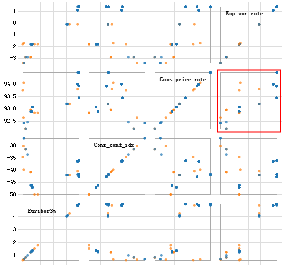
Set the label column to y. Select emp_var_rate, cons_price_rate, cons_conf_idx, and euribor3m as the feature columns.
-
Results
The chart shows the distribution of classification labels among the features.