EXPLAIN and EXPLAIN ANALYZE
Use EXPLAIN and EXPLAIN ANALYZE to inspect how Hologres executes a SQL query. When a query performs poorly or returns unexpected results, these commands show the execution plan so you can identify bottlenecks and tune your SQL or table design.
Execution plans in Hologres V1.3.4x and later are clearer and more readable. This document is based on V1.3.4x. Upgrade your instance to V1.3.4x or later to follow along.
How it works
Every SQL statement goes through two stages:
The query optimizer (QO) analyzes the query and generates an execution plan.
The query engine (QE) takes that plan, executes it, and returns the results.
The execution plan describes the operators the QE uses, the order in which data flows between them, and the estimated cost of each step. A well-chosen plan uses fewer resources and returns results faster—which is why understanding execution plans is central to SQL tuning.
Hologres is compatible with PostgreSQL and uses the same EXPLAIN / EXPLAIN ANALYZE syntax:
| Command | What it shows |
|---|---|
EXPLAIN | The QO's estimated plan. The query is not executed. |
EXPLAIN ANALYZE | The actual runtime plan. The query is executed and real timing, row counts, and memory are shown. |
Use EXPLAIN for a quick estimate. Use EXPLAIN ANALYZE for accurate diagnostics.
EXPLAIN
Syntax
EXPLAIN <sql>;Example
The following example uses a TPC-H query for illustration only and does not represent official TPC-H benchmark results.
EXPLAIN SELECT
        l_returnflag,
        l_linestatus,
        sum(l_quantity) AS sum_qty,
        sum(l_extendedprice) AS sum_base_price,
        sum(l_extendedprice * (1 - l_discount)) AS sum_disc_price,
        sum(l_extendedprice * (1 - l_discount) * (1 + l_tax)) AS sum_charge,
        avg(l_quantity) AS avg_qty,
        avg(l_extendedprice) AS avg_price,
        avg(l_discount) AS avg_disc,
        count(*) AS count_order
FROM
        lineitem
WHERE
        l_shipdate <= date '1998-12-01' - interval '120' day
GROUP BY
        l_returnflag,
        l_linestatus
ORDER BY
        l_returnflag,
        l_linestatus;
Output:
QUERY PLAN
Sort  (cost=0.00..7795.30 rows=3 width=80)
  Sort Key: l_returnflag, l_linestatus
  ->  Gather  (cost=0.00..7795.27 rows=3 width=80)
        ->  Project  (cost=0.00..7795.27 rows=3 width=80)
              ->  Project  (cost=0.00..7794.27 rows=3 width=104)
                    ->  Final HashAggregate  (cost=0.00..7793.27 rows=3 width=76)
                          Group Key: l_returnflag, l_linestatus
                          ->  Redistribution  (cost=0.00..7792.95 rows=1881 width=76)
                                Hash Key: l_returnflag, l_linestatus
                                ->  Partial HashAggregate  (cost=0.00..7792.89 rows=1881 width=76)
                                      Group Key: l_returnflag, l_linestatus
                                      ->  Local Gather  (cost=0.00..7791.81 rows=44412 width=76)
                                            ->  Decode  (cost=0.00..7791.80 rows=44412 width=76)
                                                  ->  Partial HashAggregate  (cost=0.00..7791.70 rows=44412 width=76)
                                                        Group Key: l_returnflag, l_linestatus
                                                        ->  Project  (cost=0.00..3550.73 rows=584421302 width=33)
                                                              ->  Project  (cost=0.00..2585.43 rows=584421302 width=33)
                                                                    ->  Index Scan using Clustering_index on lineitem  (cost=0.00..261.36 rows=584421302 width=25)
                                                                          Segment Filter: (l_shipdate <= '1998-08-03 00:00:00+08'::timestamp with time zone)
                                                                          Cluster Filter: (l_shipdate <= '1998-08-03 00:00:00+08'::timestamp with time zone)
Reading the output
Read the plan from bottom to top. Each -> is a node. Data flows upward from leaf nodes (the actual data sources) to the root node (the final output).
Each node shows three optimizer estimates:
| Field | Description |
|---|---|
cost | Estimated operator runtime shown as startup_cost..total_cost. The startup cost is the cost before the first output row is produced. The total cost is the cost if the operator runs to completion. A parent node's cost includes all its children. For example, Final HashAggregate (cost=0.00..7793.27) has a startup cost of 0.00 and a total cost of 7793.27. |
rows | Estimated number of output rows, based on table statistics. For scan operations, the default estimate is 1000. If you see rows=1000, statistics are likely stale—run ANALYZE <tablename> to refresh them. |
width | Estimated average row width in bytes. Larger values indicate wider output rows. |
EXPLAIN ANALYZE
Syntax
EXPLAIN ANALYZE <sql>;Example
EXPLAIN ANALYZE SELECT
        l_returnflag,
        l_linestatus,
        sum(l_quantity) AS sum_qty,
        sum(l_extendedprice) AS sum_base_price,
        sum(l_extendedprice * (1 - l_discount)) AS sum_disc_price,
        sum(l_extendedprice * (1 - l_discount) * (1 + l_tax)) AS sum_charge,
        avg(l_quantity) AS avg_qty,
        avg(l_extendedprice) AS avg_price,
        avg(l_discount) AS avg_disc,
        count(*) AS count_order
FROM
        lineitem
WHERE
        l_shipdate <= date '1998-12-01' - interval '120' day
GROUP BY
        l_returnflag,
        l_linestatus
ORDER BY
        l_returnflag,
        l_linestatus;
Output:
QUERY PLAN
Sort  (cost=0.00..7795.30 rows=3 width=80)
  Sort Key: l_returnflag, l_linestatus
[id=21 dop=1 time=2427/2427/2427ms rows=4(4/4/4) mem=3/3/3KB open=2427/2427/2427ms get_next=0/0/0ms]
  ->  Gather  (cost=0.00..7795.27 rows=3 width=80)
      [20:1 id=100003 dop=1 time=2426/2426/2426ms rows=4(4/4/4) mem=1/1/1KB open=0/0/0ms get_next=2426/2426/2426ms]
        ->  Project  (cost=0.00..7795.27 rows=3 width=80)
            [id=19 dop=20 time=2427/2426/2425ms rows=4(1/0/0) mem=87/87/87KB open=2427/2425/2425ms get_next=1/0/0ms]
              ->  Project  (cost=0.00..7794.27 rows=0 width=104)
                    ->  Final HashAggregate  (cost=0.00..7793.27 rows=3 width=76)
                          Group Key: l_returnflag, l_linestatus
                        [id=16 dop=20 time=2427/2425/2424ms rows=4(1/0/0) mem=574/570/569KB open=2427/2425/2424ms get_next=1/0/0ms]
                          ->  Redistribution  (cost=0.00..7792.95 rows=1881 width=76)
                                Hash Key: l_returnflag, l_linestatus
                              [20:20 id=100002 dop=20 time=2427/2424/2423ms rows=80(20/4/0) mem=3528/1172/584B open=1/0/0ms get_next=2426/2424/2423ms]
                                ->  Partial HashAggregate  (cost=0.00..7792.89 rows=1881 width=76)
                                      Group Key: l_returnflag, l_linestatus
                                    [id=12 dop=20 time=2428/2357/2256ms rows=80(4/4/4) mem=574/574/574KB open=2428/2357/2256ms get_next=1/0/0ms]
                                      ->  Local Gather  (cost=0.00..7791.81 rows=44412 width=76)
                                          [id=11 dop=20 time=2427/2356/2255ms rows=936(52/46/44) mem=7/6/6KB open=0/0/0ms get_next=2427/2356/2255ms pull_dop=9/9/9]
                                            ->  Decode  (cost=0.00..7791.80 rows=44412 width=76)
                                                [id=8 dop=234 time=2435/1484/5ms rows=936(4/4/4) mem=0/0/0B open=2435/1484/5ms get_next=4/0/0ms]
                                                  ->  Partial HashAggregate  (cost=0.00..7791.70 rows=44412 width=76)
                                                        Group Key: l_returnflag, l_linestatus
                                                      [id=5 dop=234 time=2435/1484/3ms rows=936(4/4/4) mem=313/312/168KB open=2435/1484/3ms get_next=0/0/0ms]
                                                        ->  Project  (cost=0.00..3550.73 rows=584421302 width=33)
                                                            [id=4 dop=234 time=2145/1281/2ms rows=585075720(4222846/2500323/3500) mem=142/141/69KB open=10/1/0ms get_next=2145/1280/2ms]
                                                              ->  Project  (cost=0.00..2585.43 rows=584421302 width=33)
                                                                  [id=3 dop=234 time=582/322/2ms rows=585075720(4222846/2500323/3500) mem=142/142/69KB open=10/1/0ms get_next=582/320/2ms]
                                                                    ->  Index Scan using Clustering_index on lineitem  (cost=0.00..261.36 rows=584421302 width=25)
                                                                          Segment Filter: (l_shipdate <= '1998-08-03 00:00:00+08'::timestamp with time zone)
                                                                          Cluster Filter: (l_shipdate <= '1998-08-03 00:00:00+08'::timestamp with time zone)
                                                                        [id=2 dop=234 time=259/125/1ms rows=585075720(4222846/2500323/3500) mem=1418/886/81KB open=10/1/0ms get_next=253/124/0ms]

ADVICE:
[node id : 1000xxx] distribution key miss match! table lineitem defined distribution keys : l_orderkey; request distribution columns : l_returnflag, l_linestatus;
shuffle data skew in different shards! max rows is 20, min rows is 0

Query id:[300200511xxxx]
======================cost======================
Total cost:[2505] ms
Optimizer cost:[47] ms
Init gangs cost:[4] ms
Build gang desc table cost:[2] ms
Start query cost:[18] ms
- Wait schema cost:[0] ms
- Lock query cost:[0] ms
- Create dataset reader cost:[0] ms
- Create split reader cost:[0] ms
Get the first block cost:[2434] ms
Get result cost:[2434] ms
====================resource====================
Memory: 921(244/230/217) MB,  straggler worker id: 72969760xxx
CPU time: 149772(38159/37443/36736) ms, straggler worker id: 72969760xxx
Physical read bytes: 3345(839/836/834) MB, straggler worker id: 72969760xxx
Read bytes: 41787(10451/10446/10444) MB, straggler worker id: 72969760xxx
DAG instance count: 41(11/10/10), straggler worker id: 72969760xxx
Fragment instance count: 275(70/68/67), straggler worker id: 72969760xxx
Reading the output
The output has four sections: QUERY PLAN, ADVICE, Cost, and Resource.
QUERY PLAN
Read the plan bottom-up, same as EXPLAIN. Each node shows two lines:
Optimizer estimates
(cost=... rows=... width=...): Same meaning as inEXPLAIN.Actual runtime measurements
[id=... dop=... time=... rows=... mem=... open=... get_next=...]: Real values collected during execution.
The runtime measurement fields are:
| Field | Format | Description |
|---|---|---|
dag dop (for example, 20:20) | input:output | Ratio of input to output concurrency. Gather 21:1 combines 21 inputs into 1. Redistribution 20:20 shuffles across 20 workers. Broadcast 1:21 fans out 1 input to 21 outputs. |
id | Integer | Unique identifier for the operator node. |
dop | Integer | Degree of parallelism (dop)—the actual parallelism during execution. Matches the instance's shard count. For Local Gather, this is the number of files scanned. |
time | max/avg/min ms | Actual execution time broken into two phases: open (operator initialization, including pulling all downstream data for operators like Hash) and get_next (fetching each batch of records). |
rows | total(max/avg/min) | Rows output by the operator. A large gap between max and min indicates data skew. |
mem | max/avg/min | Memory consumed during operator execution. Not cumulative—each operator's value is independent. |
An operator'stimevalue includes the cumulative time of its child operators. To isolate a single operator's cost, subtract its child's time. Therowsandmemvalues are per-operator and not cumulative.
ADVICE
The ADVICE section lists automatic tuning suggestions derived from the current run:
Missing or mismatched distribution keys, clustering keys, or bitmap indexes (for example,
Table xxx misses bitmap index)Stale table statistics (
Table xxx Miss Stats! please run 'analyze xxx')Data skew (
shuffle data skew in different shards! max rows is 20, min rows is 0)
These suggestions are based solely on the current query. Review them against your specific workload before applying changes.
Cost breakdown
The cost section shows where query time is spent:
| Phase | Description |
|---|---|
| Total cost | Total end-to-end query time (ms). |
| Optimizer cost | Time the QO spends generating the execution plan. |
| Build gang desc table cost | Time to convert the QO's plan into the data structures used by the execution engine. |
| Init gangs cost | Time to preprocess the plan and send requests to the execution engine. |
| Start query cost | Initialization after Init gangs—covers schema alignment, locking, and setup. Broken down further: |
| — Wait schema cost | Time for the storage engine (SE) and frontend (FE) to align schema versions. High values often indicate frequent data definition language (DDL) operations on partitioned parent tables, which can slow down data writes and queries. |
| — Lock query cost | Time spent acquiring query locks. High values indicate lock contention. |
| — Create dataset reader cost | Time to create index data readers. High values may indicate cache misses. |
| — Create split reader cost | Time to open files. High values suggest metadata cache misses and high I/O overhead. |
| Get the first block cost | Time from when the Start query phase is complete until the first record batch is returned. For operators like Hash Agg that need all downstream data before producing output, this closely matches the total Get result cost. |
| Get result cost | Time from when the Start query phase is complete until all results are returned. |
Resource consumption
Resource metrics use total(max/avg/min) format, where each value covers the worker with the highest consumption, the per-worker average, and the worker with the lowest consumption.
| Metric | Description |
|---|---|
| Memory | Total memory consumed, plus per-worker max/avg/min. |
| CPU time | Total CPU time across all cores (ms, approximate). Reflects overall query complexity. |
| Physical read bytes | Data read from disk. Occurs when results are not cached. |
| Read bytes | Total data read, including both physical reads and cache hits. |
| Affected rows | Rows affected. Shown for DML statements only. |
| DAG instance count | Number of directed acyclic graph (DAG) instances. Higher values indicate more parallelism and complexity. |
| Fragment instance count | Number of fragment instances. Higher values indicate more execution plan segments and files. |
| straggler_worker_id | ID of the worker node with the maximum resource consumption for each metric. |
Operator reference
The table below lists every operator and its role. For details and tuning guidance, see the sections that follow.
| Operator | Category | What it does |
|---|---|---|
| Seq Scan | Scan | Full table scan—no index used. |
| Seq Scan on Partitioned Table | Scan | Scans a partitioned table; shows how many partitions are selected. |
| Index Scan (Clustering_index) | Scan | Column-store scan that hits an index (segment, clustering, or bitmap). |
| Index Seek (pk_index) | Scan | Row-store scan using a primary key index. |
| Foreign Table Type | Scan | Indicates the source of a foreign table: MaxCompute, OSS, or Hologres. |
| Filter | Filter | Applies a WHERE condition that did not hit any index. |
| Segment Filter | Filter | Condition matched a segment index (Event Time Column). |
| Cluster Filter | Filter | Condition matched a clustering index. |
| Bitmap Filter | Filter | Condition matched a bitmap index. |
| Join Filter | Filter | Additional filtering applied after a join. |
| Hash Join (variants) | Join | Joins two tables using a hash table built from the smaller table. |
| Nested Loop | Join | Iterates the inner table for each outer row. Expensive for large datasets. |
| Merge Join | Join | Joins two pre-sorted inputs on the join keys. |
| Cross Join | Join | Optimized non-equi join (V3.0+) that loads the small table into memory. |
| Materialize | Join | Buffers the inner table for a Nested Loop. |
| Broadcast | Distribution | Copies a small table to all shards for a join. |
| Redistribution | Distribution | Shuffles data across shards using hash or random distribution. |
| Local Gather | Merge | Merges data from multiple files within a single shard. |
| Gather | Merge | Merges data from multiple shards into the final result. |
| Partial HashAggregate | Aggregate | Aggregates within files and shards. |
| Final HashAggregate | Aggregate | Combines partial aggregates across shards. |
| GroupAggregate | Aggregate | Aggregates pre-sorted data without hashing. |
| Sort | Other | Orders rows by one or more keys. |
| Limit | Other | Caps the number of output rows. |
| Append | Other | Merges UNION ALL subquery results. |
| Decode | Other | Decodes or encodes text-type data to accelerate computation. |
| ExecuteExternalSQL | Other | Indicates that a function or operator fell back to PQE instead of HQE. |
| Exchange | Other | Transfers data within a shard. No action needed. |
| Forward | Other | Transfers data between HQE and PQE or SQE. |
| Project | Other | Maps columns between a subquery and its outer query. No action needed. |
Scan operators
Seq scan
A Seq Scan reads the entire table without using any index.
EXPLAIN SELECT * FROM public.holo_lineitem_100g;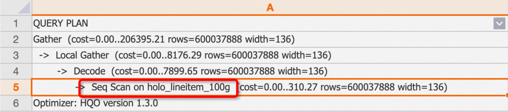
Partitioned tables show the Seq Scan on Partitioned Table operator and report "Partitions selected: x out of y":
EXPLAIN SELECT * FROM public.hologres_parent;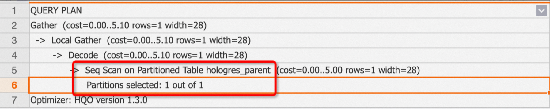
Foreign tables include a Foreign Table Type label that identifies the source (MaxCompute, OSS, or Hologres):
EXPLAIN SELECT * FROM public.odps_lineitem_100;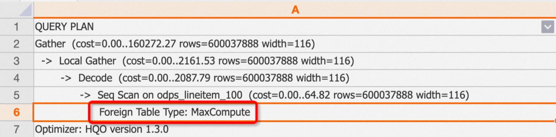
Index Scan and Index Seek
Hologres uses different index operators depending on the table's storage format:
Index Scan (Clustering_index): Used for column-store tables. Appears when a query matches an index. The plan shows sub-operators that identify which index was used: Segment Filter (segment index), Cluster Filter (clustering index), or Bitmap Filter (bitmap index). For more information, see Column store principles. Example 1: Query hits the clustering index.
BEGIN;
CREATE TABLE column_test (
 "id" bigint not null ,
 "name" text not null ,
 "age" bigint not null
);
CALL set_table_property('column_test', 'orientation', 'column');
CALL set_table_property('column_test', 'distribution_key', 'id');
CALL set_table_property('column_test', 'clustering_key', 'id');
COMMIT;

INSERT INTO column_test VALUES(1,'tom',10),(2,'tony',11),(3,'tony',12);

EXPLAIN SELECT * FROM column_test WHERE id>2;
Example 2: Query on a non-indexed column—no Clustering_index in the plan.
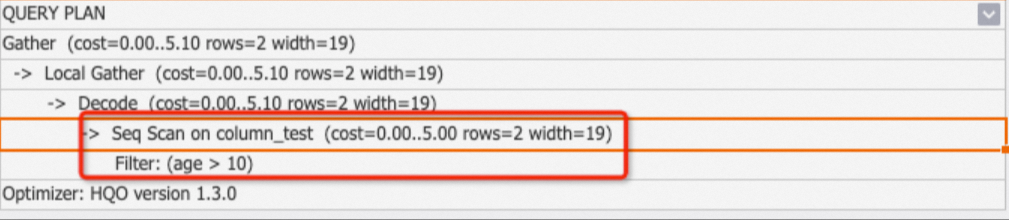
EXPLAIN SELECT * FROM column_test WHERE age>10;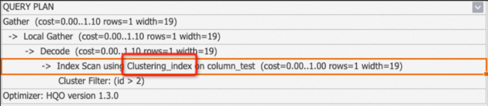
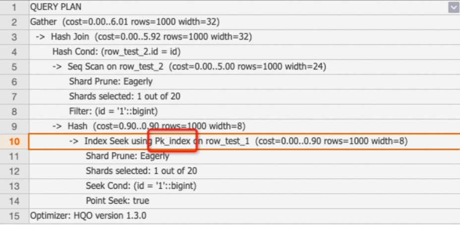
Index Seek (pk_index): Used for row-store tables with primary key indexes. Appears when a primary key query does not use Fixed Plan. For more information, see Row store principles.
BEGIN;
CREATE TABLE row_test_1 (
    id bigint not null,
    name text not null,
    class text ,
PRIMARY KEY (id)
);
CALL set_table_property('row_test_1', 'orientation', 'row');
CALL set_table_property('row_test_1', 'clustering_key', 'name');
COMMIT;
INSERT INTO row_test_1 VALUES ('1','qqq','3'),('2','aaa','4'),('3','zzz','5');

BEGIN;
CREATE TABLE row_test_2 (
    id bigint not null,
    name text not null,
    class text ,
PRIMARY KEY (id)
);
CALL set_table_property('row_test_2', 'orientation', 'row');
CALL set_table_property('row_test_2', 'clustering_key', 'name');
COMMIT;
INSERT INTO row_test_2 VALUES ('1','qqq','3'),('2','aaa','4'),('3','zzz','5');

--primary key index
EXPLAIN SELECT * FROM (SELECT id FROM row_test_1 WHERE id = 1) t1 JOIN row_test_2 t2 ON t1.id = t2.id;
Filter operators
Filter operators appear as child nodes of scan operators and indicate whether a condition matched an index.
Filter
A plain Filter means the condition did not match any index. Check the table's index configuration and add appropriate indexes to improve performance.
If the plan shows One-Time Filter: false, the result set is empty.BEGIN;
CREATE TABLE clustering_index_test (
"id" bigint not null ,
"name" text not null ,
"age" bigint not null
);
CALL set_table_property('clustering_index_test', 'orientation', 'column');
CALL set_table_property('clustering_index_test', 'distribution_key', 'id');
CALL set_table_property('clustering_index_test', 'clustering_key', 'age');
COMMIT;
INSERT INTO clustering_index_test VALUES (1,'tom',10),(2,'tony',11),(3,'tony',12);
EXPLAIN SELECT * FROM clustering_index_test WHERE id>2;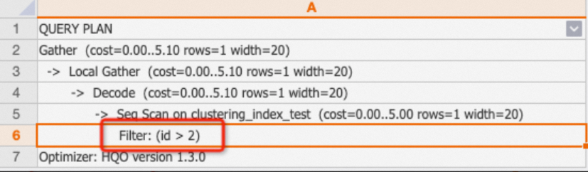
Segment Filter
The query matched a segment index (Event Time Column). Appears alongside Index Scan. See Event Time Column (segment key).
Cluster Filter
The query matched a clustering index. See Clustering key.
Bitmap Filter
The query matched a bitmap index. See Bitmap index.
Join Filter
Applies additional filtering after a join operation.
Decode
The Decode operator decodes or encodes text and similar data types to accelerate computation.
Local Gather and Gather
Data in Hologres is stored as files within shards. Local Gather merges data from multiple files within a single shard. Gather merges data from multiple shards into the final result.
EXPLAIN SELECT * FROM public.lineitem;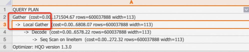
Redistribution
The Redistribution operator shuffles data across shards using hash or random distribution. It typically appears in these situations:
JOIN,COUNT DISTINCT, orGROUP BYqueries where distribution keys are missing or mismatched—data must be shuffled across shards instead of joined locally. In multi-table joins, Redistribution means local join was not used, which degrades performance.JOINorGROUP BYkeys that use expressions (such as casts) that change the original field type, which prevents local joins.
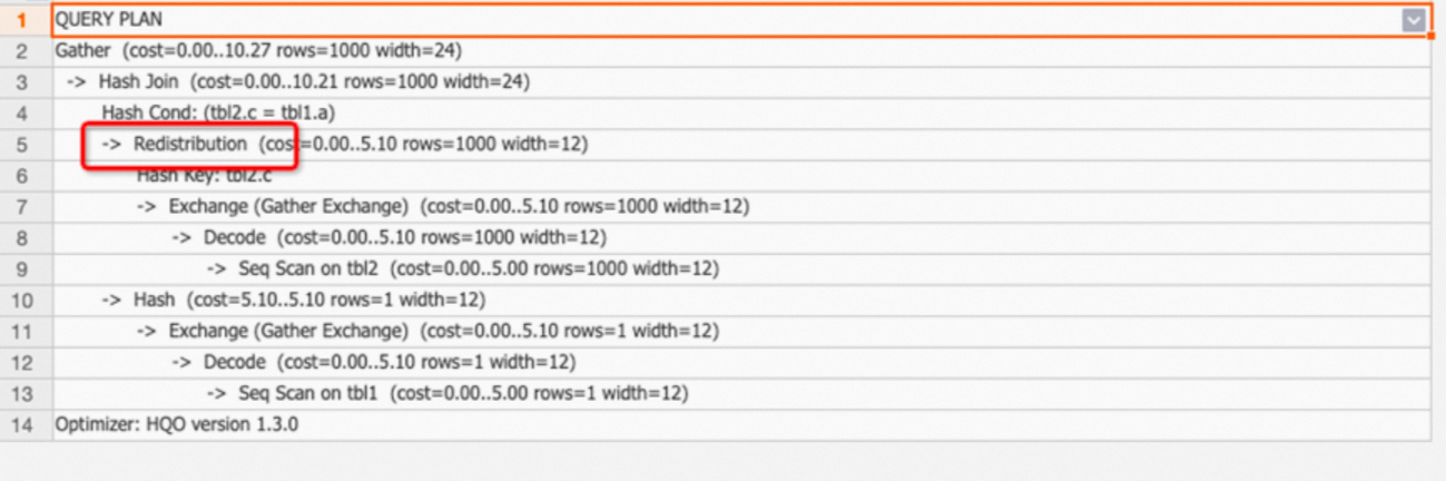
Example 1: Mismatched distribution keys cause Redistribution.
BEGIN;
CREATE TABLE tbl1(
a int not null,
b text not null
);
CALL set_table_property('tbl1', 'distribution_key', 'a');
CREATE TABLE tbl2(
c int not null,
d text not null
);
CALL set_table_property('tbl2', 'distribution_key', 'd');
COMMIT;

EXPLAIN SELECT * FROM tbl1  JOIN tbl2 ON tbl1.a=tbl2.c;
The join condition is tbl1.a=tbl2.c, but the distribution keys are a and d—a mismatch that forces a data shuffle.
If Redistribution appears, check whether distribution keys are set correctly. See Distribution key.
Example 2: A join key with a type-changing expression prevents local joins.
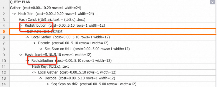
Avoid expressions on join keys to prevent this.
Join operators
Hash Join
A Hash Join builds a hash table in memory from the smaller table, then probes it row by row with data from the larger table.
| Type | Description |
|---|---|
| Hash Left Join | Returns all rows from the left table, with nulls for unmatched right table columns. |
| Hash Right Join | Returns all rows from the right table, with nulls for unmatched left table columns. |
| Hash Inner Join | Returns only rows that satisfy the join condition. |
| Hash Full Join | Returns all rows from both tables, with nulls on the non-matching side. |
| Hash Anti Join | Returns rows from the driving table that have no match—used for NOT EXISTS. |
| Hash Semi Join | Returns one row per match from the driving table—used for EXISTS. No duplicates. |
When analyzing a Hash Join, also check:
hash cond: The join condition, for examplehash cond (tmp.a=tmp1.b).hash key: The key used for hash calculation across shards, typically theGROUP BYkey.
The smaller table must be the hash table. To verify, look for the table labeled hash in the plan—reading bottom-up, it appears as the lower branch. Using the larger table as the hash table consumes excessive memory.
Tuning: update statistics
Outdated statistics cause the QO to misjudge table sizes. For example, statistics show rows=1000 for a table that actually has 1 million rows, causing the wrong table to be selected as the hash table.
BEGIN ;
CREATE TABLE public.hash_join_test_1 (
a integer not null,
b text not null
);
CALL set_table_property('public.hash_join_test_1', 'distribution_key', 'a');
CREATE TABLE public.hash_join_test_2 (
c integer not null,
d text not null
);
CALL set_table_property('public.hash_join_test_2', 'distribution_key', 'c');
COMMIT ;
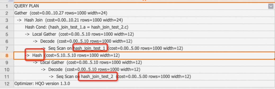
INSERT INTO hash_join_test_1 SELECT i, i+1 FROM generate_series(1, 10000) AS s(i);
INSERT INTO hash_join_test_2 SELECT i, i::text FROM generate_series(10, 1000000) AS s(i);
EXPLAIN SELECT * FROM hash_join_test_1 tbl1 JOIN hash_join_test_2 tbl2 ON tbl1.a=tbl2.c;The plan incorrectly uses the larger hash_join_test_2 as the hash table:
After refreshing statistics, the plan correctly selects the smaller table:
ANALYZE hash_join_test_1;
ANALYZE hash_join_test_2;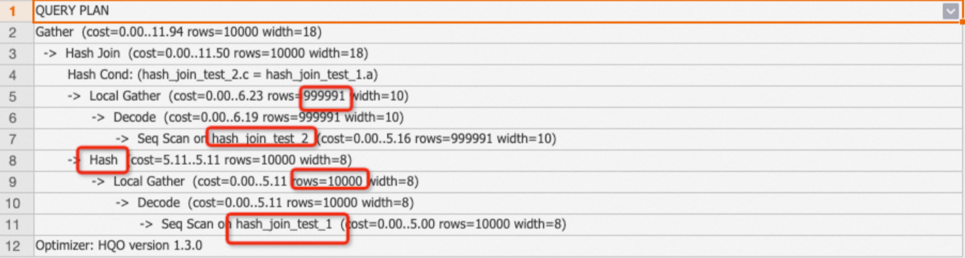
Tuning: adjust join order for complex queries
Refreshing statistics resolves most join order issues. For complex joins with five or more tables, the QO may spend significant time finding the optimal plan. Use the optimizer_join_order Grand Unified Configuration (GUC) parameter to control this:
SET optimizer_join_order = '<value>';| Value | Description |
|---|---|
exhaustive (default) | Evaluates all join order permutations. Produces optimal plans but increases optimizer overhead for many tables. |
query | Uses the join order as written in the SQL. Reduces QO overhead for joins with small tables (under 100 million rows). Do not set this at the database level—it affects all joins. |
greedy | Uses a greedy algorithm to find a good join order with moderate QO overhead. |
Nested Loop Join and Materialize
A Nested Loop operator reads the outer table row by row and searches the inner table for each match—essentially a Cartesian product. The inner table typically shows a Materialize operator in the plan.
BEGIN;
CREATE TABLE public.nestedloop_test_1 (
    a integer not null,
    b integer not null
);
CALL set_table_property('public.nestedloop_test_1', 'distribution_key', 'a');
CREATE TABLE public.nestedloop_test_2 (
    c integer not null,
    d text not null
);
CALL set_table_property('public.nestedloop_test_2', 'distribution_key', 'c');
COMMIT;

INSERT INTO nestedloop_test_1 SELECT i, i+1 FROM generate_series(1, 10000) AS s(i);
INSERT INTO nestedloop_test_2 SELECT i, i::text FROM generate_series(10, 1000000) AS s(i);

EXPLAIN SELECT * FROM nestedloop_test_1 tbl1,nestedloop_test_2 tbl2 WHERE tbl1.a>tbl2.c;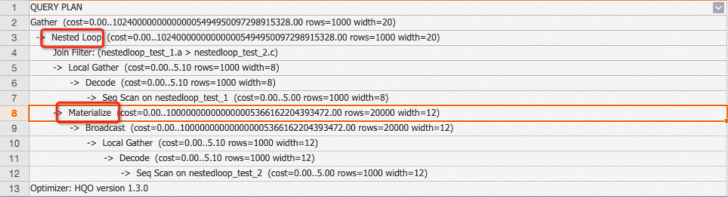
To reduce Nested Loop cost:
Keep the outer result set small to limit how many times the inner table is scanned.
Avoid non-equi joins where possible—they typically produce Nested Loop plans.
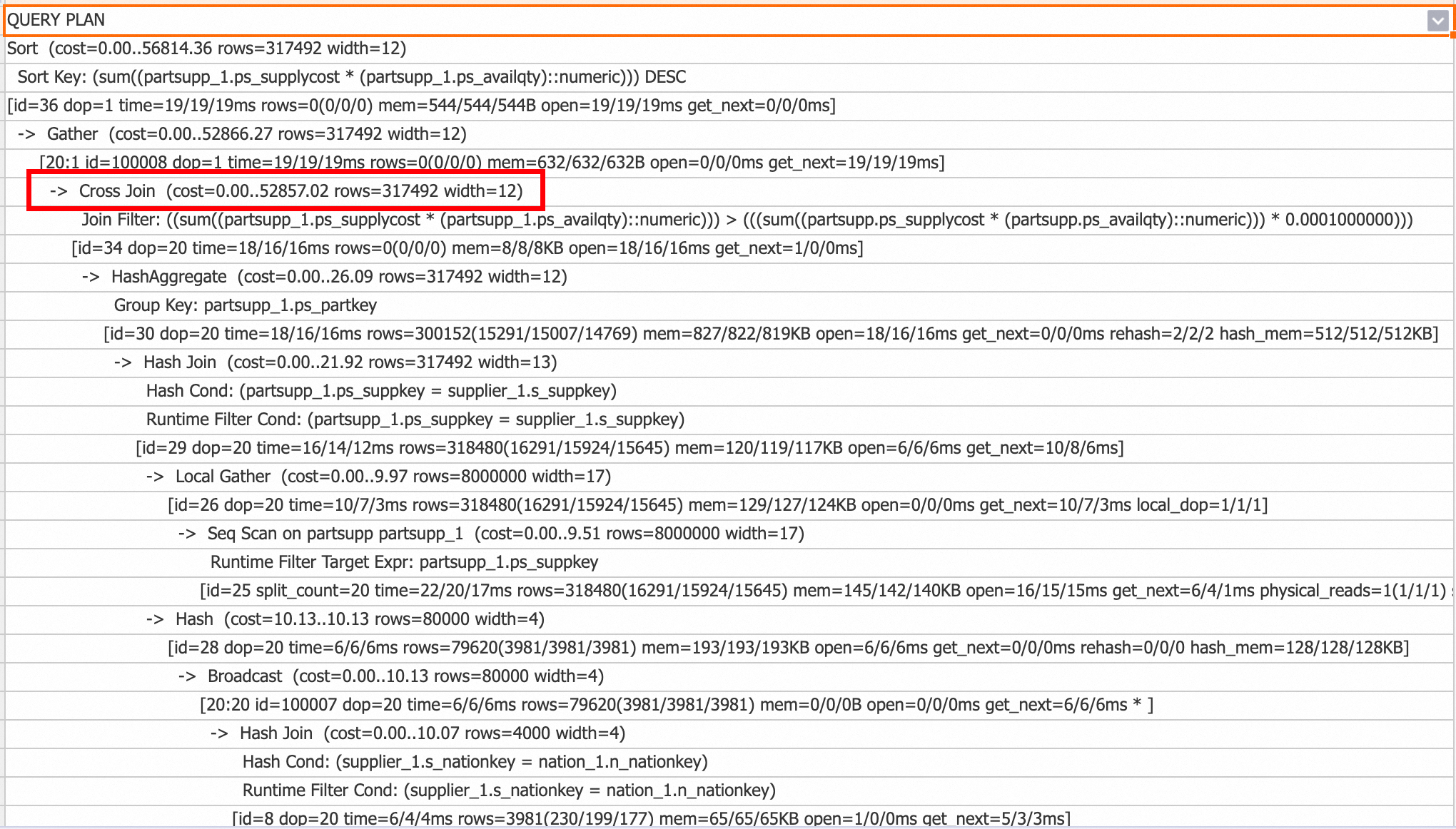
Cross Join
Starting from V3.0, the Cross Join operator optimizes non-equi join scenarios involving a small table. Unlike Nested Loop, which resets the inner state for each outer row, Cross Join loads the entire small table into memory and streams the large table through it. This is significantly faster but uses more memory.
To disable Cross Join:
-- Disable for the current session
SET hg_experimental_enable_cross_join_rewrite = off;

-- Disable at the database level (takes effect for new connections)
ALTER database <database name> hg_experimental_enable_cross_join_rewrite = off;
Merge Join
A Merge Join requires its inputs to be pre-sorted on the join keys. Hologres may select Merge Join for queries where the input data is already ordered.
Broadcast
The Broadcast operator copies a table to all shards and is used in Broadcast Join scenarios where a small table is joined with a large table. The QO compares the cost of Broadcast against Redistribution and picks the cheaper option.
Broadcast is cost-effective when the table is small and the instance has few shards (for example, 5 shards).
BEGIN;
CREATE TABLE broadcast_test_1 (
    f1 int,
    f2 int);
CALL set_table_property('broadcast_test_1','distribution_key','f2');
CREATE TABLE broadcast_test_2 (
    f1 int,
    f2 int);
COMMIT;

INSERT INTO broadcast_test_1 SELECT i AS f1, i AS f2 FROM generate_series(1, 30)i;
INSERT INTO broadcast_test_2 SELECT i AS f1, i AS f2 FROM generate_series(1, 30000)i;

ANALYZE broadcast_test_1;
ANALYZE broadcast_test_2;

EXPLAIN SELECT * FROM broadcast_test_1 t1, broadcast_test_2 t2 WHERE t1.f1=t2.f1;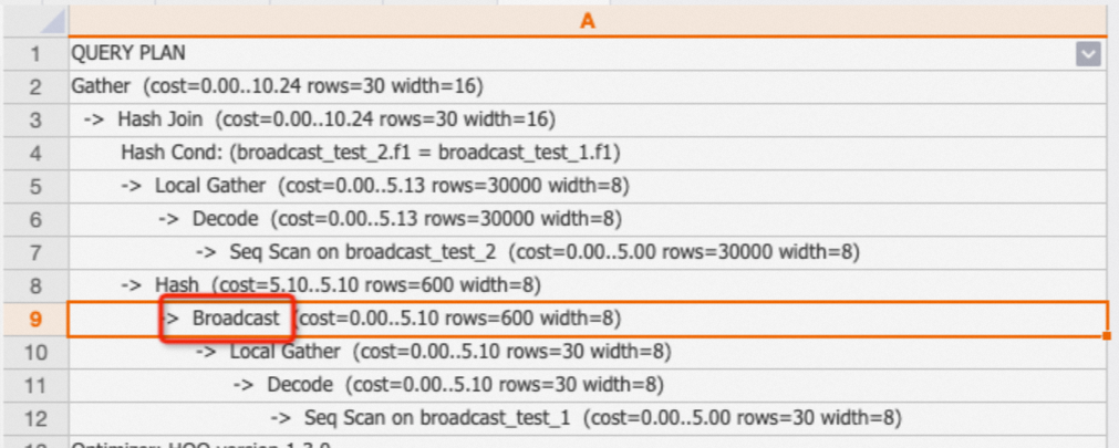
If Broadcast appears for a table that is not small, stale statistics are the likely cause (for example, statistics show 1,000 rows but the actual table has 1 million rows). Run ANALYZE <tablename> to refresh them.
Shard prune and Shards selected
Shard prune: Shows how the QO selects relevant shards. The QO chooses the appropriate method automatically.
lazily: Shards are marked by ID first and selected during computation.eagerly: Only matching shards are selected immediately; irrelevant shards are skipped.
Shards selected: The number of shards used. For example, 1 out of 20 means 1 shard was selected from 20 total.
ExecuteExternalSQL
Hologres has three query engine components: Hologres Query Engine (HQE), PostgreSQL Query Engine (PQE), and Shard Query Engine (SQE). HQE is the proprietary engine. When HQE does not support a function or operator, PQE handles it—at a performance cost. The ExecuteExternalSQL operator in a plan marks PQE execution.
Example 1: The ::timestamp cast is handled by PQE.
CREATE TABLE pqe_test(a text);
INSERT INTO pqe_test VALUES ('2023-01-28 16:25:19.082698+08');
EXPLAIN SELECT a::timestamp FROM pqe_test;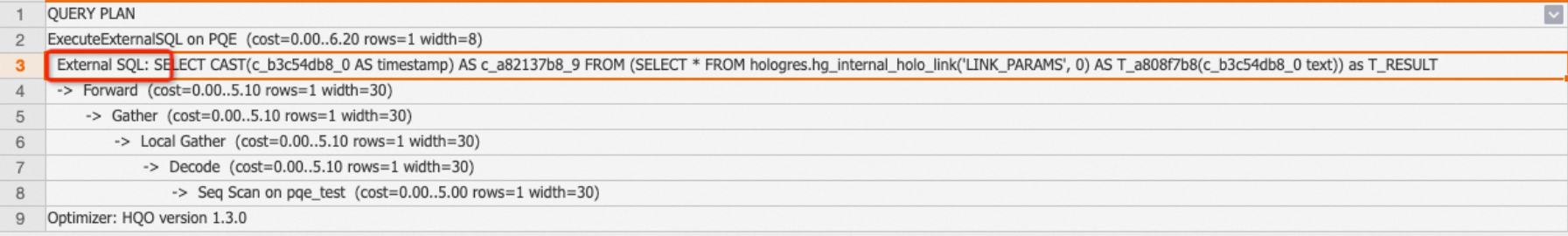
Example 2: Rewriting ::timestamp as to_timestamp uses HQE instead—no ExecuteExternalSQL in the plan.
EXPLAIN SELECT to_timestamp(a,'YYYY-MM-DD HH24:MI:SS') FROM pqe_test;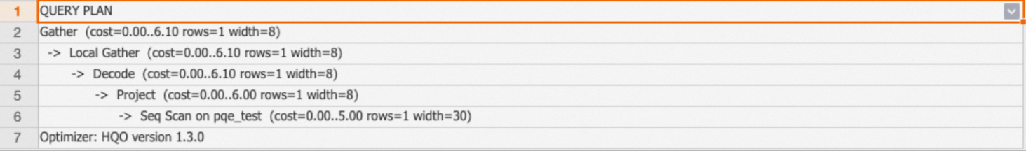
Identify functions that trigger PQE in execution plans, then rewrite them to use HQE-compatible equivalents. See Optimize query performance for common rewrite examples.
Hologres pushes more PQE operations to HQE with each release. Some functions may automatically use HQE after an upgrade. See Function release notes.
Aggregate operators
Hologres uses HashAggregate for most aggregations. HashAggregate distributes data across shards for parallel aggregation, then merges results with Gather.
For large datasets, Hologres uses multi-stage HashAggregate:
Partial HashAggregate: Aggregates within files and shards.
Final HashAggregate: Combines partial results across shards.
GroupAggregate is used when data is pre-sorted on the GROUP BY keys.
EXPLAIN SELECT
        sum(l_extendedprice * l_discount) AS revenue
FROM
        lineitem
WHERE
        l_shipdate >= date '1996-01-01'
        AND l_shipdate < date '1996-01-01' + interval '1' year
        AND l_discount BETWEEN 0.02 - 0.01 AND 0.02 + 0.01
        AND l_quantity < 24;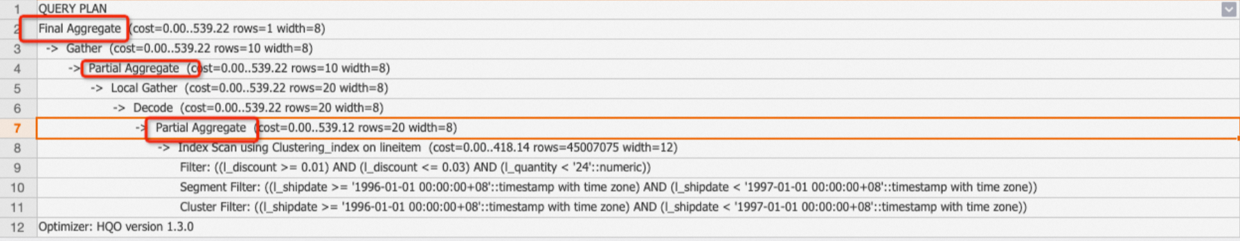
The QO automatically chooses single-stage or multi-stage HashAggregate based on data volume. If EXPLAIN ANALYZE shows high time for an Aggregate operator but the QO chose only shard-level aggregation, force multi-stage aggregation:
SET optimizer_force_multistage_agg = on;Sort
The Sort operator orders rows in ascending (ASC) or descending (DESC) order, typically from ORDER BY clauses.
EXPLAIN SELECT l_shipdate FROM public.lineitem ORDER BY l_shipdate;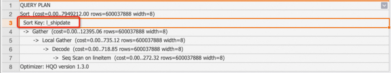
Large sort operations consume significant resources. Avoid sorting large datasets when possible.
Limit
The Limit operator caps the number of output rows. It controls only the final output, not how many rows are scanned. Check whether Limit is pushed down to the Seq Scan node to understand the actual scan volume.
EXPLAIN SELECT * FROM public.lineitem limit 1;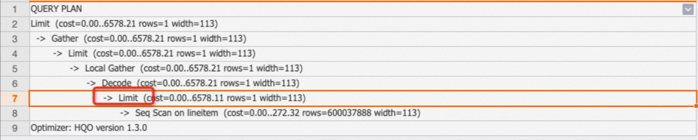
Notes on Limit:
Not all Limit operators are pushed down. Add filter conditions to reduce scanned rows.
Avoid very large LIMIT values (hundreds of thousands or more)—they increase scan time even when pushed down.
Append
The Append operator merges results from UNION ALL subqueries.
Exchange
The Exchange operator transfers data within a shard. No action is required.
Forward
The Forward operator transfers data between HQE and PQE or SQE. It appears in plans that use HQE+PQE or HQE+SQE combinations.
Project
The Project operator represents column mapping between a subquery and its outer query. No action is required.
Common performance issues
Use this section as a quick reference when you see a specific symptom in the execution plan.
| Symptom | Likely cause | What to do |
|---|---|---|
rows=1000 on a scan | Stale statistics | Run ANALYZE <tablename> |
| Redistribution on a join | Distribution key mismatch or type-changing expression on the join key | Align distribution keys with join keys; avoid expressions on join keys. See Distribution key. |
| Large table is the hash table in Hash Join | Stale statistics | Run ANALYZE on both tables |
| High Aggregate time with only shard-level aggregation | Data volume too large for single-stage aggregation | Set optimizer_force_multistage_agg = on |
| ExecuteExternalSQL appears | Function or operator not supported by HQE, falling back to PQE | Rewrite the expression to use an HQE-compatible function. See Optimize query performance. |
| Nested Loop on large tables | Non-equi join condition | Rewrite to equi-join where possible; keep the outer result set small |
High open time on Hash operators | Hash table build is slow—large inner table or slow child nodes | Check statistics and child operator times; consider join order |
Large gap between max and min rows or mem | Data skew across shards | Check ADVICE section; adjust distribution keys |
| High Wait schema cost | Frequent DDL on partitioned parent tables | Reduce DDL frequency |
| High Lock query cost | Lock contention | Investigate concurrent queries |
What's next
To visualize execution plans in HoloWeb, see View execution plans.