Simple Log Service provides the Scheduled SQL feature. You can use the feature to automatically analyze data at a scheduled time and aggregate data for storage. You can also use the feature to project and filter data. This topic describes the background information, features, terms, scheduling and running scenarios, and usage notes of Scheduled SQL.
Background information
Time-related data such as logs and metrics can accumulate to excessively large amounts. For example, if 10 million data records are generated per day, a total of approximately 3.6 billion data records are accumulated per year. Long-term data retention requires large storage. If you shorten the data retention period to reduce the required storage, your storage costs can be reduced. However, this may result in the loss of valuable data. In addition, large amounts of data can deteriorate analysis performance.
Data storage and analysis have the following requirements:
Most metrics are time sensitive. Historical data can have minute or hour precision, but new data must have higher precision.
Data users such as data operations specialists and data scientists must store full data for analysis.
The processing of full data and quick response time need to be balanced during data analysis.
To meet the preceding requirements, Simple Log Service provides the Scheduled SQL feature. You can use the feature to compress high-precision historical data to low-precision data and store the compressed data for a long term. After you enable the Scheduled SQL feature, you can change the data retention period of a source logstore or Metricstore to a smaller value such as 15 days based on your business requirements and change the data retention period of a destination logstore or Metricstore to permanent. This helps reduce the latency when long-lived data is analyzed and reduce the storage costs.
Features
Scheduled SQL supports SQL-92 syntax and the syntax of Simple Log Service query statements. Scheduled SQL jobs periodically run based on scheduling rules and write the running results to destination logstores or Metricstores.
Scheduled data analysis: You can write SQL statements or query statements based on your business requirements to perform scheduled data analysis and store the analysis results to destination logstores or Metricstores.
Global aggregation: You can aggregate full and fine-grained data for storage. This process involves lossy compression of data. The storage size and data precision after compression must meet the requirements. Examples:
If you aggregate 3.6 billion data records for storage based on the second precision, a total of 31.5 million data records are stored, and the storage size is 0.875% of the full data.
If you aggregate 3.6 billion data records for storage based on the minute precision, a total of 525,000 data records are stored, and the storage size is 0.015% of the full data.

Projection and filtering: You can filter raw data by field based on specific conditions and store the obtained data to destination logstores or Metricstores.
You can also project and filter data by using the data transformation feature, which uses the Domain Specific Language (DSL) syntax. The DSL syntax provides higher extract, transform, and load (ETL) capabilities than the SQL syntax. For more information, see How it works.
Terms
Job: Each Scheduled SQL task corresponds to a job. A job includes information such as calculation and scheduling configurations.
Instance: A Scheduled SQL job generates instances based on scheduling configurations. Each instance performs SQL calculation on raw data and writes the calculation results to the destination logstore or Metricstore.
Instance ID: the unique identifier of an instance.
Creation time: the time when an instance is created. In most cases, an instance is created based on the scheduling rules that you configure. If historical data needs to be processed or if latency exists and needs to be offset, an instance is immediately created.
Start time: the time when an instance starts to run. If a job is retried, the start time is the time when the last instance of the job starts to run.
End time: the time when an instance stops running. If a job is retried, the end time is the time when the last instance of the job stops running.
Scheduled time: the time for which a job is scheduled. The scheduled time for an instance is generated based on the scheduling rules of the job regardless of whether the previous instance times out, is delayed, or runs to process historical data.
In most cases, the scheduled time for instances that are successively generated is consecutive, and the successive instances can process a complete dataset.
SQL time window: the time range of data that is analyzed when a Scheduled SQL job runs. Simple Log Service does not analyze data beyond the time range when the job runs. An SQL time window is a left-closed and right-open interval that is calculated based on the scheduled time for an instance. An SQL time window is independent of the creation time and start time of an instance. For example, if the scheduled time for an instance is 2021/01/01 10:00:00 and the expression of the SQL time window is [@m - 10m, @m), the SQL time window of the instance is [2021/01/01 09:50:00, 2021/01/01 10:00:00).
Status: the status of a Scheduled SQL instance. An instance can be in the RUNNING, STARTING, SUCCEEDED, or FAILED state.
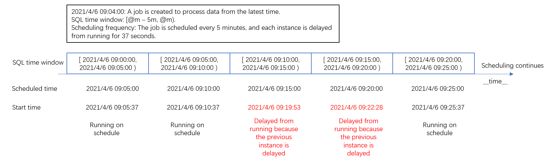
Delayed running: a parameter that you can configure for a Scheduled SQL job. If you set the parameter to N, the instance starts to run after N seconds from the scheduled time. This helps prevent inaccurate calculation results that may be caused by data latency. If you do not need to delay running an instance, you can set the Delay Task parameter to 0 Seconds.
For example, if you set the Specify Scheduling Interval parameter to Hourly and the Delay Task parameter to 30 Seconds, 24 instances are generated per day. If the scheduled time for an instance is 2021/4/6 12:00:00, the start time of the instance is 2021/4/6 12:00:30.
Scheduling and running scenarios
Each job can generate multiple instances. Only one instance of a job can be in the RUNNING state at a time, regardless of whether the job is normally scheduled or an instance is retried due to an exception. Multiple instances cannot run at the same time. The following examples illustrate the typical scenarios of scheduling and running:
Scenario 1: Delay running an instance
The scheduled time for an instance is generated in advance based on the scheduling rules of the job, regardless of whether the instance is delayed from running. If an instance is delayed, the subsequent instances may also be delayed. However, the delay can be gradually offset by running subsequent instances at a higher speed until an instance runs on schedule.
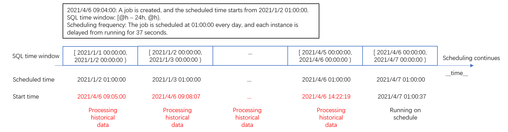
Scenario 2: Schedule a Scheduled SQL job from a historical point in time
When you create a Scheduled SQL job, you can configure scheduling rules to allow the job to process historical data. When the job is scheduled for the start historical point in time, an instance is generated to process historical data. Then, more instances are generated to process historical data. The instances run in sequence to process historical data until an instance runs on schedule.
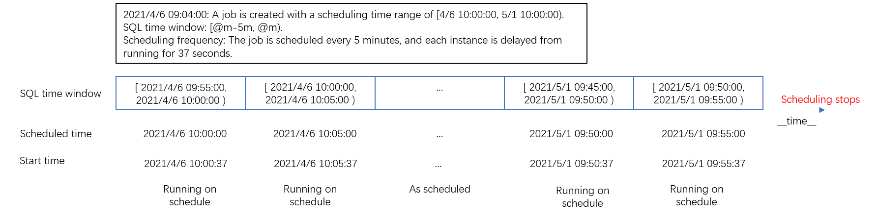
Scenario 3: Schedule a Scheduled SQL job within a specified period of time
If you want to schedule a job to process logs within a period of time, you can specify the period for scheduling. If you specify the end time for scheduling, the job does not generate instances after the last instance runs. The scheduled time for the last instance cannot be the same as or later than the end time for scheduling.
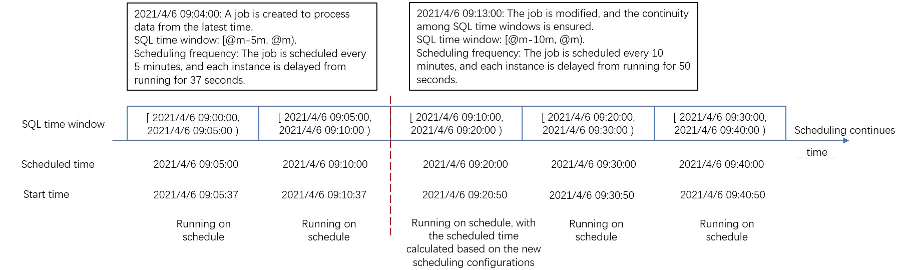
Scenario 4: Modify scheduling configurations
After you modify the scheduling configurations of a job, the job generates an instance based on the new configurations. If you want to ensure the continuity of SQL time windows among instances, you can modify the SQL time window and scheduling frequency of the scheduling configurations.
Scenario 5: Retry a failed instance
In most cases, a Scheduled SQL job generates instances in chronological order based on scheduled time. If an instance fails to run due to insufficient permissions, nonexistent source logstore or Metricstore, nonexistent destination logstore or Metricstore, or invalid SQL syntax, the system allows the instance to automatically retry. If the number of retries exceeds the upper limit that you specify or the instance is retried for a period that exceeds the maximum time that you specify, the instance stops retrying and enters the FAILED state. The next instance starts to run.
You can configure alerts for failed instances and manually retry the instances. You can view and retry the instances that are generated within the last seven days. After the instances run, the system changes the status of the instances to SUCCEEDED or FAILED based on the retry results. For more information, see Retry an instance of a Scheduled SQL job.
Usage notes
When you use the Scheduled SQL feature, we recommend that you balance the timeliness and accuracy of data based on your business requirements.
When data is uploaded to Simple Log Service, latency may exist. In this case, the data for an SQL time window may not be completely uploaded to Simple Log Service when an instance is running. To prevent this issue, we recommend that you configure the Delay Task and SQL Time Window parameters based on the data collection latency and the maximum result viewing latency allowed for your business. In addition, we recommended that you specify values that are slightly earlier than theoretical values to ensure that instances can run as expected.
To ensure the accuracy of processing results in case some unordered data is uploaded, we recommend that you specify minute- or hour-level SQL time windows for jobs.