DataWorks:Configure a single-table real-time sync task

1. Configure the source

1. On the Configuration tab, select the Kafka topic that you want to synchronize.

   Use the default settings or modify them as needed. For more information about the parameters, see the official Kafka documentation.

2. In the upper-right corner, click Data Sampling.

   In the dialog box that appears, specify the Start time and Sampled Data Records, and then click Start Collection. This samples data from the specified Kafka topic. You can preview the data in the topic, which provides input for the data preview and visual configuration in subsequent data processing nodes.

3. On the Configure Output Field tab, select the fields that you want to synchronize.

   Kafka provides six default fields.

   Field name	Description
   __key__	The key of the Kafka record.
   __value__	The value of the Kafka record.
   __partition__	The partition number where the Kafka record is stored. Partition numbers are integers that start from 0.
   __headers__	The headers of the Kafka record.
   __offset__	The offset of the Kafka record in its partition. Offsets are integers that start from 0.
   __timestamp__	The 13-digit integer millisecond timestamp of the Kafka record.

   You can also perform more field transformations in subsequent data processing steps.

2. Process data

Turn on Data Processing. Five processing methods are available: Data Masking, String Replace, Data Filtering, JSON Parsing, and Edit and assign fields. Arrange these methods in your desired order of execution.

After you configure a data processing step, you can click Preview Data Output in the upper-right corner:

1. The table under the input data shows the results from the previous Data Sampling step. Click Re-obtain Output of Ancestor Node to refresh the results.

2. If there is no output from the upstream step, you can use Manually Construct Data to simulate the upstream output.

3. Click Preview to view the output data from the upstream step after it has been processed by the data processing component.

3. Configure the destination

1. In the Destination section, select a Tunnel resource group. By default, Public Transfer Resource is selected, which uses the free quota of MaxCompute.

2. Choose whether to write data to a new table or an existing table.

   1. If you choose to create a new table, select Create from the drop-down list. By default, a table with the same schema as the data source is created. You can manually change the destination table name and schema.

   2. If you choose to use an existing table, select the target table from the drop-down list.

3. (Optional) Edit the Table Schema.

   Click the edit icon next to the table name to edit the Table Schema. You can click Re-generate Table Schema Based on Output Column of Ancestor Node to automatically generate a Table Schema based on the output columns from the upstream node. You can select a column in the auto-generated schema to be the primary key.

Synchronization tasks provide advanced parameters for fine-grained control. In most cases, you do not need to change the default values. If necessary, you can:

1. Click Advanced Parameters in the upper-right corner to go to the Advanced Parameters configuration page.

   Note

   The advanced parameters are on a tab on the right side of the task configuration page.

2. You can set parameters separately for the reader and writer of the sync task. To customize the Runtime Configuration, disable Auto-configure Runtime Settings.

3. Modify parameter values as described in the tooltips. For parameter descriptions, refer to the explanations next to the parameter names. For configuration recommendations for some parameters, see Advanced parameters for real-time synchronization.

1. Add an alert

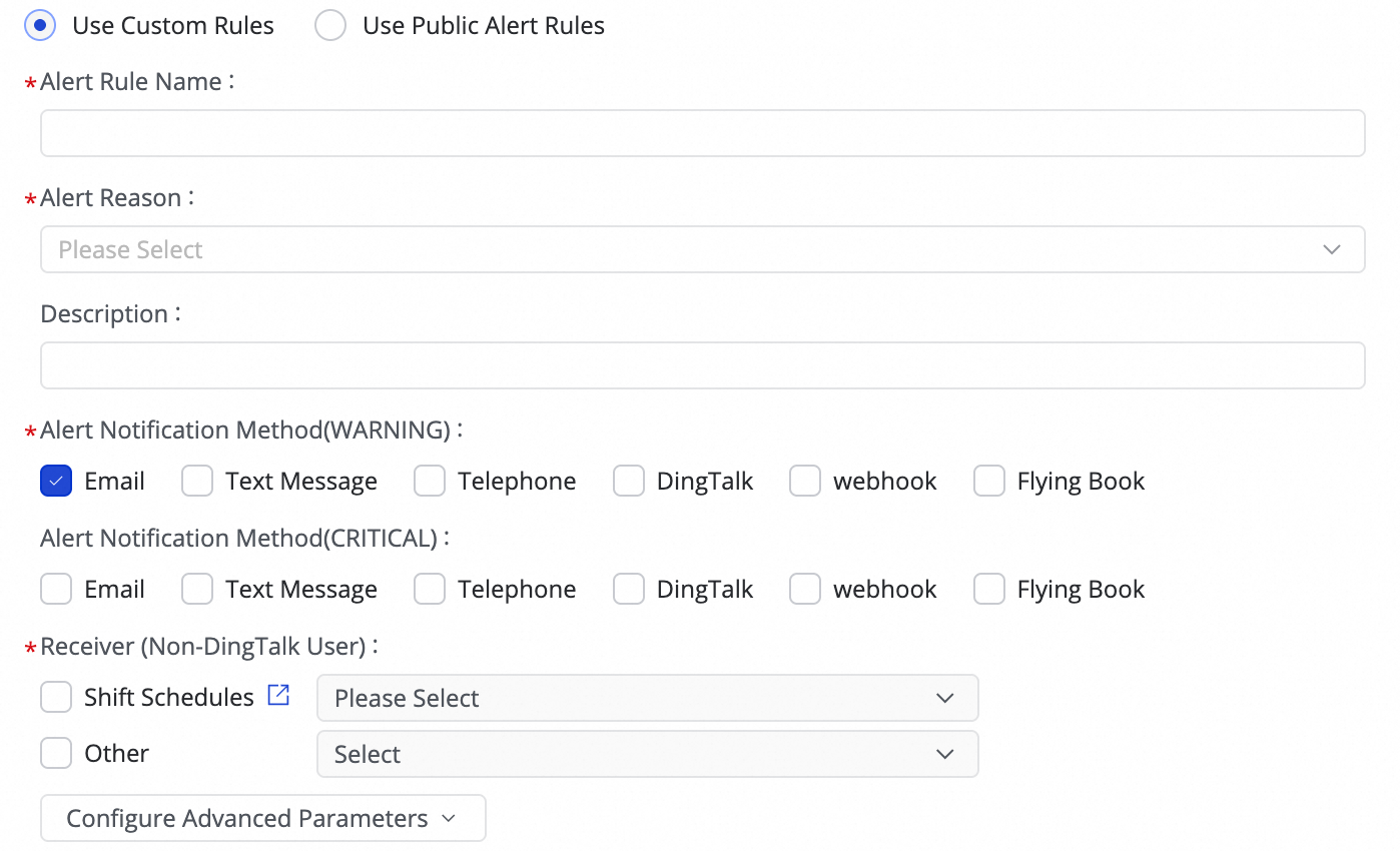
(1) Click Create Rule to configure the Alert Rule.

You can set Alert Reason to monitor metrics such as Business delay, failover, Task status, DDL Notification, and Task Resource Utilization. You can set CRITICAL or WARNING alert levels based on specified thresholds.

• After setting the alert method, you can use Configure Advanced Parameters to control the interval for sending alert messages. This prevents sending too many messages at once, which can cause waste and message backlog.

• If you select Business delay, Task status, or Task Resource Utilization as the alert trigger, you can also enable recovery notifications to inform recipients when the task returns to normal.

(2) Manage Alert Rules.

For existing Alert Rules, you can use the alert switch to enable or disable them. You can also notify different contacts based on the alert level.

2. View alerts

Click More > Configure Alert Rule for the task to view a history of alert events.