:DataWorks OpenLake one-stop intelligent data lakehouse development

Introduction to DataWorks

DataWorks is an intelligent platform for data lakehouse development and governance. It is built on 15 years of Alibaba's big data construction methodology. It is deeply integrated with dozens of Alibaba Cloud big data and AI computing services, such as MaxCompute, E-MapReduce, Hologres, Flink, and PAI. DataWorks provides intelligent extract, transform, and load (ETL) development, data analysis, and proactive data asset governance services for data warehouses, data lakes, and OpenLake data lakehouse architectures. This helps you manage the entire "Data+AI" lifecycle. Since 2009, DataWorks has continuously productized Alibaba's data architecture. It serves various industries, including government, finance, retail, the Internet, automotive, and manufacturing. Tens of thousands of customers use DataWorks to drive digital transformation and create value.

Introduction to DataWorks Copilot

DataWorks Copilot is your intelligent assistant in DataWorks. In DataWorks, you can choose to use the DataWorks default model, Qwen3-235B-A22B, DeepSeek-R2-0528, or the Qwen3-Coder large model to perform Copilot operations. With the deep inference capabilities of DeepSeek-R2, DataWorks Copilot helps you perform complex operations such as SQL code generation, optimization, and testing through natural language interaction. This significantly improves ETL development and data analysis efficiency.

Introduction to DataWorks Notebook

DataWorks Notebook is an intelligent, interactive tool for data development and analysis. It supports SQL or Python analysis across multiple data engines. You can run or debug code instantly and view visualized data results. A DataWorks Notebook can also be orchestrated with other task nodes into a workflow and submitted to the scheduling system for execution. This lets you flexibly implement complex business scenarios.

Step 1: Manage the data catalog

The data catalog management feature of the data lakehouse lets you manage and create data catalogs for services such as DLF, MaxCompute, and Hologres.

1. In DataStudio, click the icon in the left-side menu to open Data Catalog. In the navigation pane, find the metadata type that you want to manage and click Add Project. The name of this button may vary depending on the metadata type. This topic uses MaxCompute as an example.

   You can add data sources from your DataWorks workspace. You can also select a MaxCompute project for which you have permissions on the MaxCompute-Project tab.

   

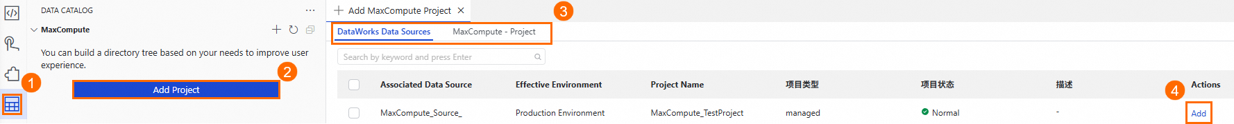
2. After you add the project, it appears under the corresponding metadata type. Click the project name to go to the data catalog details page.

3. On the data catalog details page, select a schema and click any table name to view the table details.

4. The data catalog lets you create tables visually.

   Expand the data catalog to the Table level of the specified schema. Click the icon on the right to open the Create Table page.

   

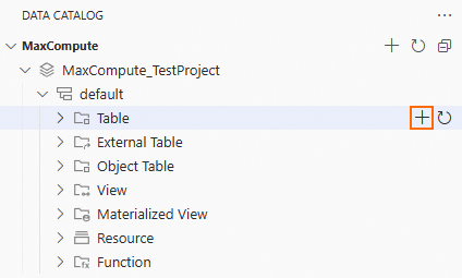
5. On the Create Table page, you can create a table in the following ways:

   • In area ①, enter the Table Name and Field Information.

   • In area ②, you can directly enter the DDL statement to create the table.

   

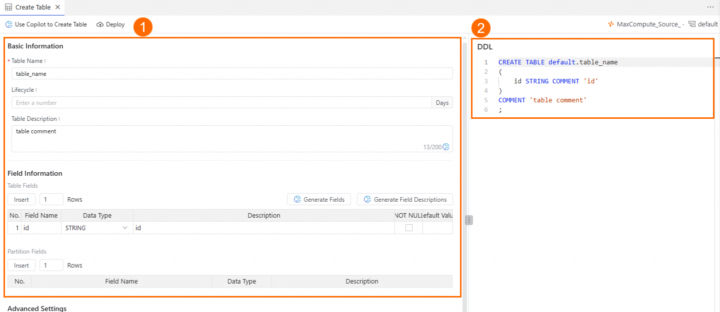
6. Click the Publish button at the top of the page to create the table.

Step 2: Orchestrate a workflow

A workflow lets you orchestrate various types of data development nodes by dragging and dropping them based on your business logic. You do not need to configure common parameters, such as scheduling time, for each node. This helps you easily manage complex task projects.

1. In DataStudio, click the icon in the primary menu on the left to open Data Development. In the navigation pane on the left, find Project Folder, click the icon next to it, and select New Workflow.

2. Enter a Name for the workflow and click OK to open the workflow editor.

3. In the workflow editor, click Drag Or Click To Add A Node on the canvas. In the Add Node dialog box, set Node Type to Zero Load Node, enter a custom Node Name, and then click Confirm.

4. From the list of node types on the left, find the required node type and drag it onto the canvas. In the Add Node dialog box, enter a Node Name and click Confirm.

   

5. On the canvas, find the two nodes for which you want to create a dependency. Hover your mouse over the middle of the bottom edge of one node. When the pointer changes to a +, drag the arrow to the other node and release the mouse. After you set the dependency as shown in the figure, click Save on the top toolbar.

   

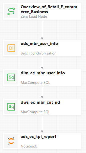
6. After clicking Save, you can adjust the canvas layout as needed.

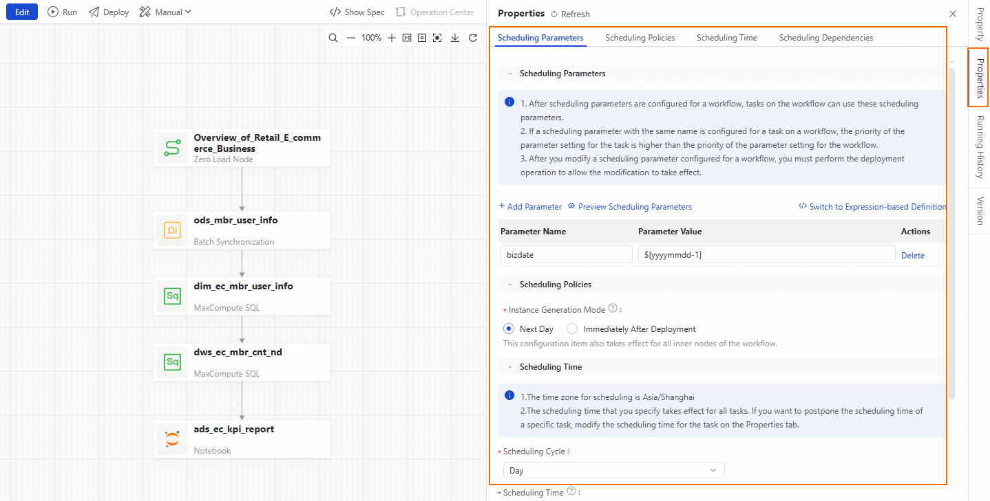
7. On the right side of the workflow canvas, click Scheduling Configuration. Use the Scheduling Configuration panel to configure the scheduling parameters and node dependencies for the workflow. In the Scheduling Parameters section, click Add Parameter. In the parameter name field, enter bizdate. From the parameter value drop-down list, select $[yyyymmdd-1].

   

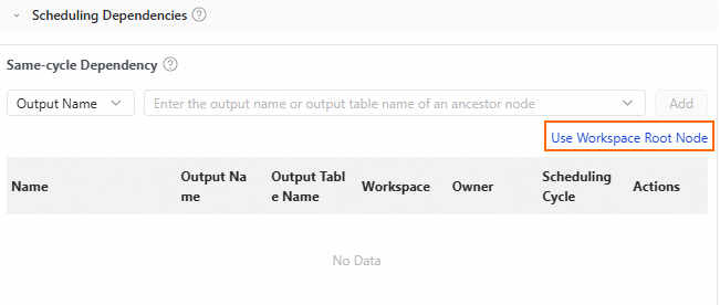
8. Click Use Workspace Root Node to set this node as the upstream dependency for the workflow.

   

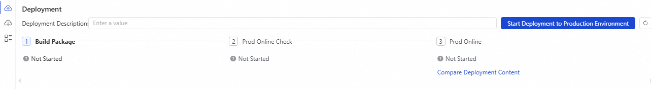
9. Click Publish above the workflow canvas. The Publish Content panel appears in the lower-right corner. In the panel, click Start Publishing To Production and follow the prompts to confirm.

   

Step 3: Use multi-engine collaborative development

DataStudio supports data warehouse development for dozens of node types across different engines, such as Data Integration, MaxCompute, Hologres, EMR, Flink, Python, Notebook, and ADB. It supports complex scheduling dependencies and provides a development model that isolates the development environment from the production environment. This experiment uses the creation of a Flink SQL Streaming node as an example.

1. In DataStudio, click the icon in the navigation pane on the left to open the Data Development page. In the navigation pane, find Project Folder and click the icon next to it. In the cascading menu, click Flink SQL Streaming to open the node editor. Before the editor opens, enter a Node Name and press Enter.

   Preset node name: ads_ec_page_visit_log.

   

2. In the node editor, paste the preset Flink SQL Stream code into the code editor.

   

   Preset Flink SQL Stream code

   CREATE TEMPORARY VIEW log_ri_base
   AS 
   SELECT 
     visit_time
     ,substring(visit_time,1,8) as stat_date
     ,substring(visit_time,9,2) as stat_hour
     ,visitor_id
     ,item_id
     ,cate_id
     ,ext_pv
   FROM vvp_ec_ads.dws_log_all_itm_ipv_ri
   WHERE
     bc_type IN ('b', 'z')
     AND coalesce(cate_id, '') <> ''
     AND visitor_type = 'uid'
     and coalesce(item_id, '') <> ''
     AND substring(visit_time,1,8) >= '${bizdate}'
   ;
   
   
   CREATE TEMPORARY VIEW itm_log_day
   AS
   SELECT
     sum(ext_pv) as pv
     ,count(DISTINCT visitor_id) FILTER (WHERE ext_pv>0) as uv
     ,stat_date
     ,cate_id
     ,item_id
   FROM log_ri_base
   GROUP BY stat_date
     ,cate_id
     ,item_id
   ;
   
   
   CREATE TEMPORARY VIEW itm_log_hh_00
   AS
   SELECT
     sum(ext_pv) as pv
     ,count(DISTINCT visitor_id) FILTER (WHERE ext_pv>0) as uv
     ,stat_date
     ,stat_hour
     ,item_id
     ,cate_id
   FROM log_ri_base
   GROUP BY stat_date
     ,stat_hour
     ,cate_id
     ,item_id
   ;
   
   BEGIN STATEMENT SET;
   
   INSERT INTO vvp_ec_ads.ads_ec_log
   SELECT
     a.stat_date
     ,cast(a.item_id as varchar) as item_id
     ,a.cate_id
     ,b.cate_name
     ,cast(b.industry_id as varchar) as industry_id
     ,cast(b.xcat1_id as varchar) as xcat1_id
     ,cast(b.xcat2_id as varchar) as xcat2_id
     ,cast(b.xcat3_id as varchar) as xcat3_id
     ,cast(b.cate_level1_id as varchar) as cate_level1_id
     ,cast(b.cate_level2_id as varchar) as cate_level2_id
     ,cast(b.is_sw as varchar) as is_sw
     ,a.pv as mbr_ipv_1d
     ,a.uv as mbr_ipv_uv_1d
     ,DATE_FORMAT(CURRENT_TIMESTAMP,'yyyy-MM-dd HH:mm:ss') as log_gmt_modify
     ,DATE_FORMAT(CURRENT_TIMESTAMP,'yyyy-MM-dd HH:mm:ss') as gmt_modify
   FROM itm_log_day a
   JOIN ec.dim_tm_cate_360_2pt_ri FOR SYSTEM_TIME AS OF PROCTIME() AS b
   ON vvp_dt_rtcdm.DateAddOrSub(a.stat_date, -2) = b.stat_date 
       AND a.cate_id = b.cate_id
   ;
   
   --Write
   INSERT INTO vvp_ec_ads.ads_ec_log_hh
   
   SELECT
     a.stat_date
     ,a.stat_hour
     ,cast(a.item_id as varchar) as item_id
     ,a.cate_id
     ,b.cate_name
     ,cast(b.industry_id as varchar) as industry_id
     ,cast(b.xcat1_id as varchar) as xcat1_id
     ,cast(b.xcat2_id as varchar) as xcat2_id
     ,cast(b.xcat3_id as varchar) as xcat3_id
     ,cast(b.cate_level1_id as varchar) as cate_level1_id
     ,cast(b.cate_level2_id as varchar) as cate_level2_id
     ,cast(b.is_sw as varchar) as is_sw
     ,a.pv as mbr_ipv_1h
     ,a.uv as mbr_ipv_uv_1h
     ,DATE_FORMAT(CURRENT_TIMESTAMP,'yyyy-MM-dd HH:mm:ss') as log_gmt_modify
     ,DATE_FORMAT(CURRENT_TIMESTAMP,'yyyy-MM-dd HH:mm:ss') as gmt_modify
   FROM itm_log_hh_00 a
   JOIN ec.dim_tm_cate_360_2pt_ri FOR SYSTEM_TIME AS OF PROCTIME() AS b
   ON vvp_ec_ads.DateAddOrSub(a.stat_date, -2) = b.stat_date 
       AND a.cate_id = b.cate_id
   ;
   
   END;

3. In the node editor, click Real-time Configuration on the right side of the code editor to configure the Flink Resource Information, Script Parameters, and Flink Runtime Parameters.

   

   Preset Flink SQL Stream real-time configuration - Expert mode code

   {
     "nodes": [
       {
         "profile": {
           "parallelism": 256,
           "maxParallelism": 32768,
           "minParallelism": 1,
           "group": "0"
         },
         "id": 1,
         "type": "StreamExecTableSourceScan",
         "desc": "Source: vvp_dt_rtcdm_dwd_tb_trd_ord_pay_nrt_ri[71980]"
       },
       {
         "profile": {
           "parallelism": 256,
           "maxParallelism": 32768,
           "minParallelism": 1,
           "group": "0"
         },
         "id": 2,
         "type": "StreamExecCalc",
         "desc": "Calc[71981]"
       },
       {
         "profile": {
           "parallelism": 256,
           "maxParallelism": 32768,
           "minParallelism": 1,
           "group": "0"
         },
         "id": 3,
         "type": "StreamExecLookupJoin",
         "desc": "LookupJoin[71982]"
       },
       {
         "profile": {
           "parallelism": 256,
           "maxParallelism": 32768,
           "minParallelism": 1,
           "group": "0"
         },
         "id": 4,
         "type": "StreamExecCalc",
         "desc": "Calc[71983]"
       },
       {
         "profile": {
           "parallelism": 256,
           "maxParallelism": 32768,
           "minParallelism": 1,
           "group": "1"
         },
         "id": 6,
         "state": [
           {
             "userDefined": false,
             "name": "groupAggregateState",
             "index": 0,
             "ttl": "36 h"
           }
         ],
         "type": "StreamExecGroupAggregate",
         "desc": "GroupAggregate[71985]"
       },
       {
         "profile": {
           "parallelism": 256,
           "maxParallelism": 32768,
           "minParallelism": 1,
           "group": "1"
         },
         "id": 7,
         "type": "StreamExecCalc",
         "desc": "Calc[71986]"
       },
       {
         "profile": {
           "parallelism": 256,
           "maxParallelism": 32768,
           "minParallelism": 1,
           "group": "1"
         },
         "id": 8,
         "type": "StreamExecSink",
         "desc": "ConstraintEnforcer[71987]"
       },
       {
         "profile": {
           "parallelism": 256,
           "maxParallelism": 32768,
           "minParallelism": 1,
           "group": "2"
         },
         "id": 10,
         "state": [
           {
             "userDefined": false,
             "name": "sinkMaterializeState",
             "index": 0,
             "ttl": "36 h"
           }
         ],
         "type": "StreamExecSink",
         "desc": "SinkMaterializer[71987]"
       },
       {
         "profile": {
           "parallelism": 256,
           "maxParallelism": 32768,
           "minParallelism": 1,
           "group": "2"
         },
         "id": 11,
         "type": "StreamExecSink",
         "desc": "Sink: vvp_dt_ads_tb_dev_ads_tb_idec_seckill_cate_bc_trd_flow_htr_000[71987]"
       }
     ],
     "vertices": {
       "2d95a2974e3b3137fd533ecfd3490bc5": [
         10,
         11
       ],
       "717c7b8afebbfb7137f6f0f99beb2a94": [
         1,
         2,
         3,
         4
       ],
       "44b79c13fdb45883c7f21ee510155f4d": [
         6,
         7,
         8
       ]
     },
     "edges": [
       {
         "mode": "PIPELINED",
         "source": 1,
         "strategy": "FORWARD",
         "target": 2
       },
       {
         "mode": "PIPELINED",
         "source": 2,
         "strategy": "FORWARD",
         "target": 3
       },
       {
         "mode": "PIPELINED",
         "source": 3,
         "strategy": "FORWARD",
         "target": 4
       },
       {
         "mode": "PIPELINED",
         "source": 4,
         "strategy": "HASH",
         "target": 6
       },
       {
         "mode": "PIPELINED",
         "source": 6,
         "strategy": "FORWARD",
         "target": 7
       },
       {
         "mode": "PIPELINED",
         "source": 7,
         "strategy": "FORWARD",
         "target": 8
       },
       {
         "mode": "PIPELINED",
         "source": 8,
         "strategy": "HASH",
         "target": 10
       },
       {
         "mode": "PIPELINED",
         "source": 10,
         "strategy": "FORWARD",
         "target": 11
       }
     ],
     "ssgProfiles": [
       {
         "managed": {},
         "name": "0",
         "cpu": 0.25,
         "offHeap": "32 mb",
         "heap": "992 mb",
         "extended": {}
       },
       {
         "managed": {
           "STATE_BACKEND": "512 mb"
         },
         "name": "1",
         "cpu": 0.25,
         "offHeap": "32 mb",
         "heap": "480 mb",
         "extended": {}
       },
       {
         "managed": {
           "STATE_BACKEND": "512 mb"
         },
         "name": "2",
         "cpu": 0.25,
         "offHeap": "32 mb",
         "heap": "480 mb",
         "extended": {}
       }
     ]
   

   Preset Flink SQL Stream real-time configuration - Flink runtime parameters - Other configurations

   blob.fetch.backlog: 1000
   taskmanager.debug.memory.log-interval: 5000

4. After you configure the real-time settings, click Save above the code editor. Then click Publish. In the Publish Content panel that appears in the lower-right corner, click Start Publishing To Production and follow the prompts to confirm.

   

Step 4: Enter the personal development environment

The personal development environment supports custom container images, connecting to user NAS and Git, and programming in Python using Notebooks.

In DataStudio, click the icon at the top of the page. In the drop-down menu, select the personal development environment that you want to enter and wait for the page to load.

Step 5: Program and debug in Python

DataWorks is deeply integrated with DSW. After you enter the personal development environment, DataStudio supports writing, debugging, running, and scheduling Python code.

1. On the DataStudio page, in your personal developer environment, click the workspace folder. Click the icon to the right of Personal Folder. An untitled file appears in the list on the left. Name the file, press Enter, and wait for it to be generated.

   Preset file name: ec_item_rec.py.

   

2. In the code editor on the Python file page, enter the preset Python code. Then, click Run Python File above the code editor and check the results in the Terminal at the bottom of the page.

   

   

   Preset Python code

   import pandas as pd
   from surprise import Dataset, Reader, SVD
   from surprise.model_selection import train_test_split
   from surprise import accuracy
   
   # Create sample data
   data_dict = {
       'user_id': [1, 1, 1, 2, 2, 2, 3, 3, 4],
       'item_id': [101, 102, 103, 101, 104, 105, 102, 105, 101],
       'rating': [5, 3, 4, 2, 4, 5, 4, 5, 3]
   }
   
   # Convert the data to a DataFrame
   df = pd.DataFrame(data_dict)
   
   # Prepare the dataset using the Surprise library
   reader = Reader(rating_scale=(1, 5))
   data = Dataset.load_from_df(df[['user_id', 'item_id', 'rating']], reader)
   
   # Split the dataset into a training set and a test set
   trainset, testset = train_test_split(data, test_size=0.2)
   
   # Use the SVD algorithm for recommendations
   model = SVD()
   model.fit(trainset)
   
   # Make predictions
   predictions = model.test(testset)
   
   # Calculate RMSE
   rmse = accuracy.rmse(predictions)
   print(f'RMSE: {rmse:.2f}')
   
   # Get recommended products for a user
   def get_recommendations(user_id, model, all_items, n=3):
       item_ids = all_items['item_id'].unique()
       user_item_col = all_items[(all_items['user_id'] == user_id)]['item_id']
       unseen_items = [item for item in item_ids if item not in user_item_col.values]
   
       # Predict ratings for unseen items
       predictions = []
       for item in unseen_items:
           pred = model.predict(user_id, item)
           predictions.append((item, pred.est))
   
       # Sort by predicted rating
       predictions.sort(key=lambda x: x[1], reverse=True)
       return predictions[:n]
   
   # Get product recommendations
   all_items = df
   user_id = 1  # The ID of the user to get recommendations for
   recommendations = get_recommendations(user_id, model, all_items)
   
   print(f'Recommended products for user {user_id}:')
   for item_id, score in recommendations:
       print(f'Product ID: {item_id}, Predicted score: {score:.2f}')

   Python environment installation

   pip install pandas scikit-surprise

3. To debug the code, click Debug Python File above the code editor or click the icon in the panel to the left of the code editor. You can set breakpoints by clicking to the left of the line numbers.

   

Step 6: Explore data with a Notebook

Notebook data exploration operations are performed in the personal development environment. You must complete Step 4: Enter the personal development environment before you begin.