Boost your query speed with proven best practices. From updating statistics to refining table designs, this guide helps you quickly identify bottlenecks and ensure your Hologres instance runs at peak performance.
Quick decision guide
Symptom | Likely cause | Recommended action |
Slow joins on large internal tables | Outdated statistics | Run ANALYZE on all tables involved in the join |
Queries scan too many rows for range or equality filters | Missing clustering key, bitmap columns, or segment key | Add a clustering_key for range filters, bitmap_columns for equality filters, or a segment_key for time-based ranges |
High latency for point queries | Unsuitable storage type or missing primary key/index | Use row or hybrid storage and define an appropriate primary key and index |
Slow COUNT DISTINCT aggregations | Resource-intensive exact deduplication | Use APPROX_COUNT_DISTINCT or UNIQ, and consider using the distinct key as the distribution key |
Slow GROUP BY aggregations | Data redistribution and data skew on GROUP BY keys | Set GROUP BY keys as distribution keys where possible and fix data skew |
Maintain statistics
Statistics (e.g., data distributions, rows, columns) help the optimizer choose efficient execution plans. Outdated statistics can cause poor join order selection and OOM errors. to generate optimal execution plans.
Check if statistics are current
Run EXPLAIN on your query and check the rows estimate for each table.
If a large table shows rows=1000 (the default), the statistics are outdated.
Update statistics
Run ANALYZE on tables with stale statistics:
analyze <tablename>;Identify when to update statistics
Run the analyze <tablename> command in the following situations.
After importing data.
After multiple INSERT, UPDATE, or DELETE operations.
For both internal and foreign tables.
On parent tables for partitioned tables.
In addition, if you encounter OOM errors during joins or slow query performance, run analyze <tablename> before you run the import task to optimize efficiency.
Configure shard count
The shard count represents query execution parallelism and is critical to performance. Too few shards cause insufficient parallelism. Too many shards increase startup overhead.
Understand default shard count
Hologres sets a default shard count based on instance specifications, approximately equal to available query CUs. After instance scaling, existing databases retain their original shard count—only new databases use the updated default.
Determine when to adjust shard count
After scaling up by 5x or more: Create a new Table Group with a larger shard count.
For new business workloads: Create a new Table Group with appropriate shard count.
When experiencing parallelism issues: Check if total shards exceed the recommended default.
Total shards across all Table Groups should not exceed the instance's default shard count for optimal CPU utilization.
Optimize JOIN queries
Use the following methods to improve join performance.
Update statistics for join queries
As mentioned in Maintain statistics, outdated statistics may cause the larger table to create a hash table, reducing join efficiency. Run ANALYZE to update table statistics.
Select distribution keys for local joins
Distribution keys determine how data is distributed across shards. Proper selection enables local joins and reduces data shuffling.
Principles for selecting distribution keys:
Use join columns as the distribution key.
Use columns in frequent GROUP BY clauses
Choose columns with even, discrete data distribution
Example: When joining tables frequently on a specific column, set that column as the distribution key for both tables:
-- Create tables with matching distribution keys
BEGIN;
CREATE TABLE orders (order_id INT, customer_id INT, amount DECIMAL);
CALL set_table_property('orders', 'distribution_key', 'customer_id');
COMMIT;

BEGIN;
CREATE TABLE customers (id INT, name TEXT);
CALL set_table_property('customers', 'distribution_key', 'id');
COMMIT;
After setting distribution keys correctly, the execution plan shows no Redistribute Motion operator, indicating local joins without data shuffling.
Use Runtime Filter in joins
Starting from V2.0, Hologres automatically applies Set up runtime filter to improve join performance optimization for large-small table joins. This reduces scanned data and improves join performance without manual configuration.
Tune join order algorithms
For complex queries with many tables, the optimizer may spend significant time finding the optimal join order. Adjust the algorithm if optimization time is excessive:
set optimizer_join_order = '<value>'; Algorithm | Use case | Trade-off |
exhaustive2 | Default for most queries | Best plan, highest optimization cost |
greedy | More than 10 tables | Faster optimization, potentially suboptimal plan |
query | Simple, well-ordered SQL | Executes in SQL order, lowest optimization cost |
Optimize Motion operators in joins
Hologres uses Motion operators to redistribute data between shards:
Motion type | Description |
Redistribute Motion | Shuffles data by hash or random |
Broadcast Motion | Copies data to all shards. |
Gather Motion | Collects data to single shard. |
Forward Motion | Transfers data between external sources and Hologres for federated queries. |
Check execution plans for costly Motion operators and adjust table design accordingly:
Time-consuming Motion operators: Redesign the distribution.
Inefficient Motion characters caused by outdated statistics: Refresh statistics with
analyze.Broadcasting small tables: Reduce shard counts to optimize Broadcast Motion efficiency.
Optimize aggregations
Optimize COUNT DISTINCT
Replace exact COUNT DISTINCT (resource-intensive) with APPROX_COUNT_DISTINCT (faster, 0.1% to 1% error rate) when slight variance is acceptable.
Replace COUNT DISTINCT with UNIQ (V1.3+).
Set an appropriate distribution key
Set the Count Distinct key as the distribution key for multiple operations with the same key to avoid data shuffles.
Upgrade to V2.1+ for built-in optimizations
These versions include built-in optimizations for various COUNT DISTINCT scenarios: one or more COUNT DISTINCT, data skew, and no GROUP BY.
Force multi-stage aggregation
Multi-stage aggregation reduces data transfer by performing partial aggregations within each shard first:
set optimizer_force_multistage_agg = on;Optimize multiple aggregate functions on the same column
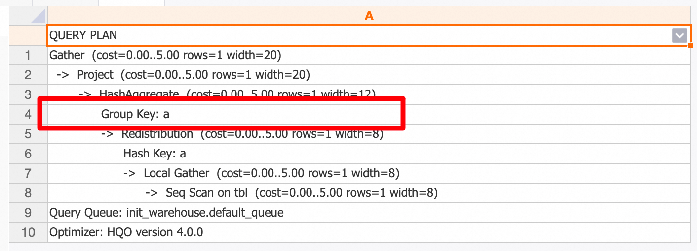
Starting from V4.0, Hologres automatically rewrites multiple identical aggregate functions on the same column to reduce calculations and improve query performance. Upgrade to V4.0+ to enjoy the enhancement.
Example:
-- Create a test table.
CREATE TABLE tbl(x int4, y int4);

-- Insert test data.
INSERT INTO tbl VALUES (1,2), (null,200), (1000,null), (10000,20000);

-- Query data
SELECT
    sum(x + 1),
    sum(x + 2),
    sum(x - 3),
    sum(x - 4)
FROM
    tbl;
The query plan shows x is the only group key.
Explicitly disable this feature using the following GUC parameter:
-- Disable at the session level.
SET hg_experimental_remove_related_group_by_key = off;

-- Disable at the DB level.
ALTER DATABASE <database_name> SET hg_experimental_remove_related_group_by_key = off;
Optimize table schema and indexes
Choose storage formats
Hologres supports row, column, and hybrid storage. Select a storage class based on your business scenario:
Storage format | Best for | Trade-off |
Row store | Point queries by primary key, frequent UPDATE/DELETE | Poor range scan and aggregation performance |
Column store | Analytics, multi-column queries, aggregations | Slower UPDATE/DELETE and point queries |
Hybrid row-columnar store | Mixed workloads | Higher storage overhead |
Choose data types
Use smaller types where possible (
INTinstead ofBIGINT)Specify precision for
DECIMAL/NUMERICtypes.Avoid
FLOATorDOUBLEforGROUP BYcolumns.Use
TEXTfor versatility. Minimize N when usingVARCHAR(N)orCHAR(N).Use
TIMESTAMPTZandDATEinstead ofTEXTfor dates.Use consistent data types in join conditions to avoid implicit conversions
Design a primary key
Primary keys ensure data uniqueness. Select a deduplication method during import:
ignore: Ignore new data.
update: Overwrite old data.
Proper primary keys improve execution plans, especially for GROUP BY queries.
Setting a primary key in columnar store scenarios can slow down writes. Performance is typically 3x faster without a primary key.
Use a partitioned table
Hologres supports single-level partitioning. Proper partitioning accelerates queries, but excessive partitions create too many small files and degrade performance.
Create daily partitions for incremental data to isolate storage and access.
Applicable scenarios:
DROP or TRUNCATE entire partitions for better performance than DELETE and no impact on other partitions.
Isolate scans to specific partitions or child tables.
Use partitioned tables for periodic real-time imports. For example, use the date as the partition key. Sample statements:
begin;
create table insert_partition(c1 bigint not null, c2 boolean, c3 float not null, c4 text, c5 timestamptz not null) partition by list(c4);
call set_table_property('insert_partition', 'orientation', 'column');
commit;
create table insert_partition_child1 partition of insert_partition for values in('20190707');
create table insert_partition_child2 partition of insert_partition for values in('20190708');
create table insert_partition_child3 partition of insert_partition for values in('20190709');

select * from insert_partition where c4 >= '20190708';
select * from insert_partition_child3;
Choose proper indexes
Hologres supports various index types. Design your table schema based on your business scenario before writing data:
Type | Purpose | Example query |
clustering_key | Range queries and filtering |
|
bitmap_columns | Equality queries |
|
segment_key (also known as event_time_column) | Time-based filtering (file-level) Provides fast initial filtering before bitmap or cluster indexing. Follows the leftmost prefix matching principle (usually 1 column). Set the first non-empty timestamp as the segment_key. |
|
Take note of the following:
Clustering and segment keys follow the leftmost prefix matching principle.
Bitmap indexes support AND/OR queries on multiple columns.
It's recommended to first use
segment_keyfor time-based filtering, and thenbitmap_columnsfor equality queries orclustering_keyfor range queries.
Example:
BEGIN;
CREATE TABLE events (
    event_id INT NOT NULL,
    user_id INT NOT NULL,
    event_time TIMESTAMPTZ NOT NULL,
    event_type TEXT
);
CALL set_table_property('events', 'clustering_key', 'event_time');
CALL set_table_property('events', 'segment_key', 'event_time');
CALL set_table_property('events', 'bitmap_columns', 'user_id,event_type');
COMMIT;
bitmap_columns can be added after table creation. clustering_key and segment_key must be specified at creation.
Verify index usage in a query by running EXPLAIN:
EXPLAIN SELECT * FROM events WHERE event_time > '2026-01-01';Disable dictionary encoding for character columns
Dictionary encoding speeds up string comparisons but adds encode/decode overhead. Disable it for columns where comparison cost is low:
BEGIN;
CREATE TABLE logs (id INT, message TEXT);
CALL set_table_property('logs', 'dictionary_encoding_columns', '');
COMMIT;
Optimize SQL statements
Avoid external SQL (Postgres) such as NOT IN
Hologres uses HQE (Hologres Query Engine) for optimal performance. When HQE doesn't support an operator, it falls back to PQE (Postgres Query Engine), reducing performance.
Checking for PQE fallback in execution plans:
EXPLAIN SELECT * FROM orders WHERE id NOT IN (SELECT id FROM cancelled_orders);If you see External SQL (Postgres), rewrite the query:
HQE-unsupported | Rewrite to | Example | Notes |
|
| | N/A. |
|
| | regexp_split_to_table supports regular expressions. Starting from Hologres V2.0.4, HQE supports |
|
| Rewrite as: | Some V0.10 versions and earlier versions of Hologres do not support substring. In V1.3 and later, HQE supports non-regular expression input parameters for the substring function. |
|
| Rewrite as: |
|
| Delete | Rewrite as: | N/A. |
|
| Rewrite as: | Supported by HQE starting from Hologres V2.0. |
|
| Rewrite as: | Supported by HQE starting from Hologres V2.0. |
Avoid fuzzy LIKE queries
Avoid fuzzy searches like the LIKE operation as they do not use indexes.
Optimize ORDER BY LIMIT queries
Starting from V1.3, Hologres supports Merge Sort for ORDER BY ... LIMIT queries, eliminating extra sort operations.
Optimize GROUP BY queries
Set the GROUP BY column as the distribution key if operations are time-consuming to reduce data redistribution.
-- If data is distributed based on the values in column a, runtime data redistribution is reduced, and the parallel computing capability of shards is fully utilized.
select a, count(1) from t1 group by a;
Starting from V4.0, Hologres automatically rewrites multiple related GROUP BY columns to reduce merges (max search depth: 5 layers). For example, a clause such as GROUP BY COL_A, ((COL_A + 1)), ((COL_A + 2)) is rewritten to the equivalent GROUP BY COL_A. For example:
CREATE TABLE tbl (
    a int,
    b int,
    c int
);

-- Query
SELECT
    a,
    a + 1 as a1,
    a + 2 as a2,
    sum(b)
FROM tbl
GROUP BY
    a,
    a1,
    a2;
The execution plan shows a query rewrite was performed, and the GROUP BY clause contains only column a.
Disable this feature using the following GUC parameter:
-- Disable the feature at the session level.
SET hg_experimental_remove_related_group_by_key = off;

-- Disable the feature at the database level.
ALTER DATABASE <database_name> SET hg_experimental_remove_related_group_by_key = off;
Enable CTE reuse
When a CTE is referenced multiple times, enable CTE reuse to avoid recomputation (V1.3+):
SET optimizer_cte_inlining=off;CTE reuse defaults to disabled. Enable it manually via GUC.
CTE reuse relies on Spill in the Shuffle stage. Large data volumes may affect performance due to varying consumption rates.
Optimize Top-N analysis
In OLAP scenarios, retrieving the top N records within a group is a common requirement. For example, the following SQL query retrieves the top two records from the
ttable within eachbpartition, sorted bya:CREATE TABLE t ( a int, b int ); INSERT INTO t VALUES (2, 1), (3, 1), (4, 1), (5, 2), (6, 2); SELECT * FROM ( SELECT a, b, row_number() OVER (PARTITION BY b ORDER BY a) AS rn FROM t) t1 WHERE rn <= 2;The execution result is as follows:
a	b	rn
5	2	1
6	2	2
2	1	1
3	1	2
In this scenario, starting from Hologres V4.1, the
Partition Sortoperator is supported. This operator supports stream sorting and pushes theLIMITclause down into thePartition. This filters data in advance during sorting, which reduces the memory consumption of sorting window functions, such asrow_numberandrank, in Top-N scenarios and lowers the probability of a query OOM error. This feature is enabled by default. You can disable it using the following GUC parameter:-- Disable the feature at the session level. SET hg_experimental_enable_hash_partitioned_sort_v2 = off; -- Disable the feature at the database level. ALTER DATABASE <database_name> SET hg_experimental_enable_hash_partitioned_sort_v2 = off;
Handle data skew
Uneven data distribution slows down queries. Detect skew by checking row counts per shard: Check for data skew using the following statement:
-- hg_shard_id is a built-in hidden column in each table that describes the shard where the corresponding row of data is located.
SELECT hg_shard_id, count(1) FROM t1 GROUP BY hg_shard_id;
If some shards have significantly more rows than others:
Change the
distribution_keyto a column with even data distribution.ImportantChanging the distribution key requires recreating the table and reimporting data.
If data is inherently skewed, optimize from a business perspective
Disable result caching for testing
Hologres caches query results by default. Disable caching when benchmarking performance:
set hg_experimental_enable_result_cache = off;