By Leimao from Cainiao Team
Today, artificial intelligence (AI) is no longer a strange idea to ordinary people. Technologies (such as intelligent voice and autonomous driving) are common ways artificial intelligence is used.
Artificial intelligence can be roughly divided into problem solving, machine learning, natural language processing (NLP), speech recognition, computer vision, and robotics. There is no strict division between these fields, and they all intersect with each other.
| Field | Description |
| Problem Solving | A broad and general field for problem solving, decision making, constraint satisfaction, and other types of inferences. Its subfields include systems, planning, automatic programming, game, and automatic inferences based on experts or knowledge. Problem solving is the most successful field of symbolic Al. |
| Machine Learning | Automatically generate new facts, concepts, or truths through rote learning, experience, or suggestions |
| Natural Language Processing (NLP) | Sentences are parsed and converted into knowledge representation (such as a semantic network), and the results are returned as sentences that are properly structured and easy to understand. As such, AI can understand and generate written human language (such as English or Japanese). |
| Speech Recognition | Transform sound waves into phones, words, and sentences and deliver them to the natural language understanding system. Perform speech synthesis converts text responses into the natural pronunciation of uses |
| Computer Vision | The pixels in the image are converted into edges, regions, textures, and geometric objects. This way, the scene can be understood, and the objects in the field of view can be finally recognized. |
| Robotics | Actuators are planned and controlled to move or manipulate objects in the real world. |
Note: AI has been developing for decades, and its development can be roughly divided into three stages.
In October 1950, Turing proposed the concept of artificial intelligence (AI). In 1966, the psychotherapy robot ELIZA (with a limited lexicon) was created.
In the second stage, people began to abandon the thinking of the symbolic school and used statistical thinking to solve problems.
The maturity of two conditions results in the advent of the third stage:
The market value of NVIDIA created by Jensen Huang has increased by 20 times over the past five years. NVIDIA has also surpassed Intel in market value for the first time after the US stock market closed on July 8, 2020, becoming the most valuable chip manufacturer in the United States. Due to the rapid development of GPUs, the problem with the computing power of artificial intelligence has finally been solved, and AI has finally ushered in a new era.
That finishes the background information. Now, let's turn our attention to today's topic: deep learning. Deep learning is a small branch of machine learning that belongs to supervised learning, one of the three machine learning categories. The other two are unsupervised learning and reinforcement learning.
First, we will discuss the basic ideas of machine learning:
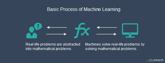
This process can be concluded into steps of modeling, parameter tuning, solving, and evaluating.
The core of the model created by machine learning is the algorithm. However, each model consists of six steps, no matter which models are created:
As for the algorithm itself, since this article focuses on deep learning, we have provided a list below:
| Linear regression | Supervised learning | Random forest | Supervised learning |
| Logistic regression | Supervised learning | AdaBoost | Supervised learning |
| Linear Discriminant Analysis | Supervised learning | Gaussian mixture model | Unsupervised learning |
| Decision tree | Supervised learning | Restricted Boltzmann machine | Unsupervised learning |
| Naive Bayes classifier | Supervised learning | k-means clustering | Unsupervised learning |
| K-nearest neighbors | Supervised learning | Expectation-maximization algorithm | Unsupervised learning |
| Learning vector quantization | Supervised learning | Random forest | Supervised learning |
| Support Vector Machine | Supervised learning |
The type of algorithm determines the type of machine learning. The key point of supervised learning is to mark all the data. This means we need to mark out the type of training data provided for the machine.
Unsupervised learning does not mark the data. Instead, computers extract features to train and classify. Finally, the data is classified by humans. The application scenarios of the two are different. Unsupervised learning is an expert on exception handling. Imagine if the bank supervises the abnormal behavior of users. Then, those operations different from normal user behaviors will be detected.
We can summarize machine learning with one sentence. Based on the specific massive amount of data, it summarizes some specific knowledge and then applies the knowledge to solve practical problems in the real scenario.
Deep learning is a supervised type of machine learning. Therefore, it has all the characteristics of supervised learning.
What are the unique characteristics of deep learning? How can we distinguish it from other types of supervised learning? The answer is neural network!
Deep learning mainly involves three types of approaches:
Convolutional neural networks are the most typical type of deep learning. It has multiple layers of nodes, which reflects its depth. Now, we will discuss the structure and knowledge points of the whole neural network. First, let's look at the figure below:

If you cannot understand it, don't worry. We can split it. Let's look at the general neural network first:
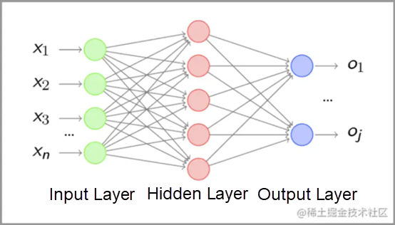
There are three layers for neural networks: input layer, hidden layer, and output layer. The points at each layer are called neurons, which contain activation values. Input and output are easy to understand. Most work of the neural network is completed in the middle: the hidden layer. The network calculates each value at the hidden layer with the bias values, the weights (W), and the activation function.
Let's learn the principle of neural networks with a sample network containing two hidden layers. First, let's look at a group of 28*28 pictures:


Humans will know these numbers soon. The input looks like pixels for human eyes. We can imitate the steps of human vision:
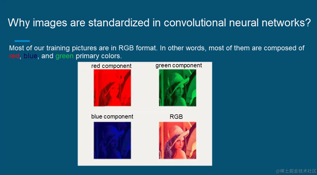
The neural network works in a similar way. A picture is composed of binary pixels for the machine. For convenience, we use zero and one to represent these pixels. (The real color pixel includes RGB color mode.)

So, we input 28*28 for the machine, namely 784 input values.
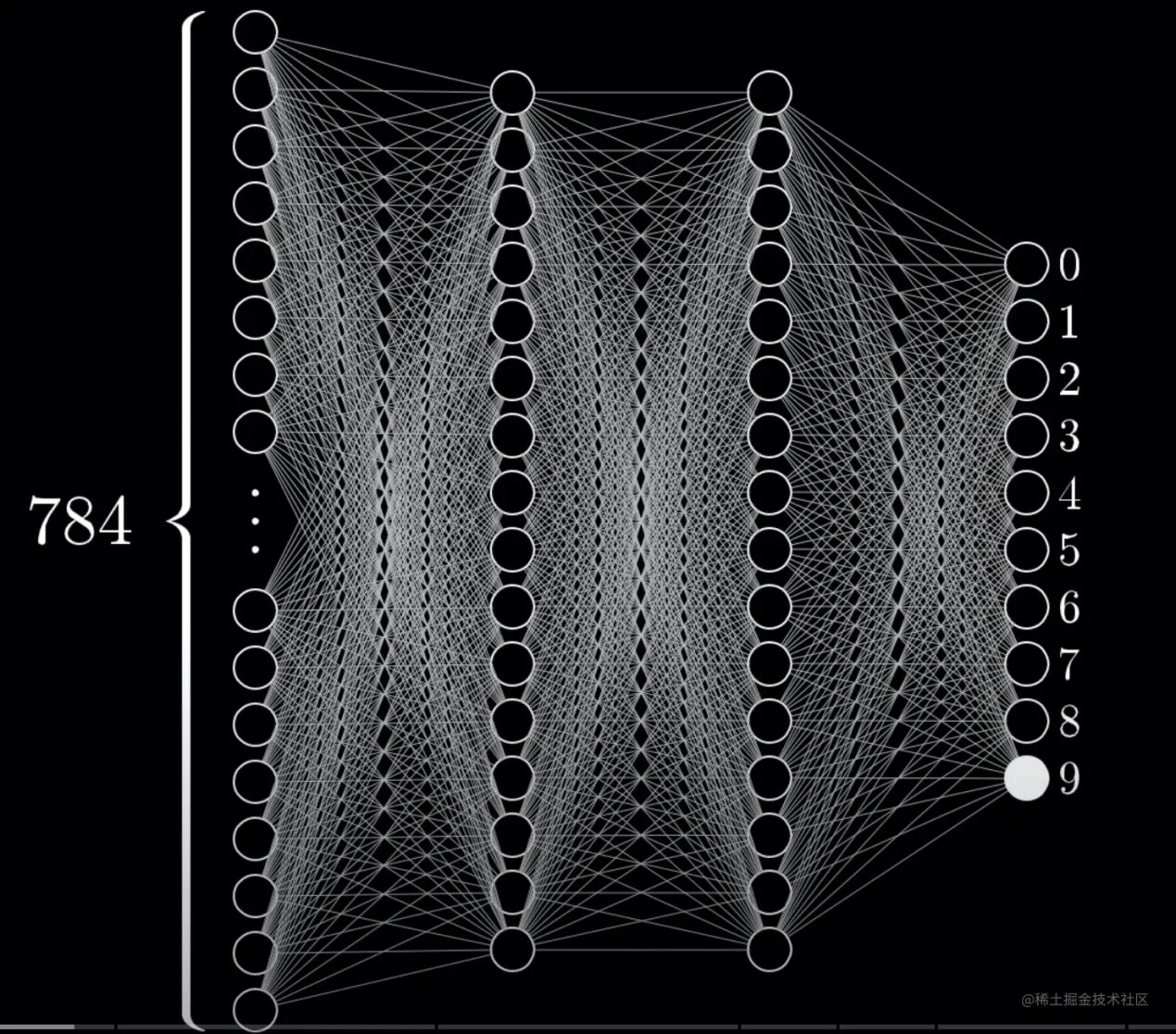
There will be output through various calculations. The result of the figure above can be identified as 9. This is the Multilayer Perception, which is the hidden layer we mentioned earlier. Do you see the lines above? They are called weights (W), and the nodes are called neurons, each with an activation value.
We will explain from the perspective of human vision to help you understand the structure. Our vision starts from edges to components to the whole. Imagine if we split a number:
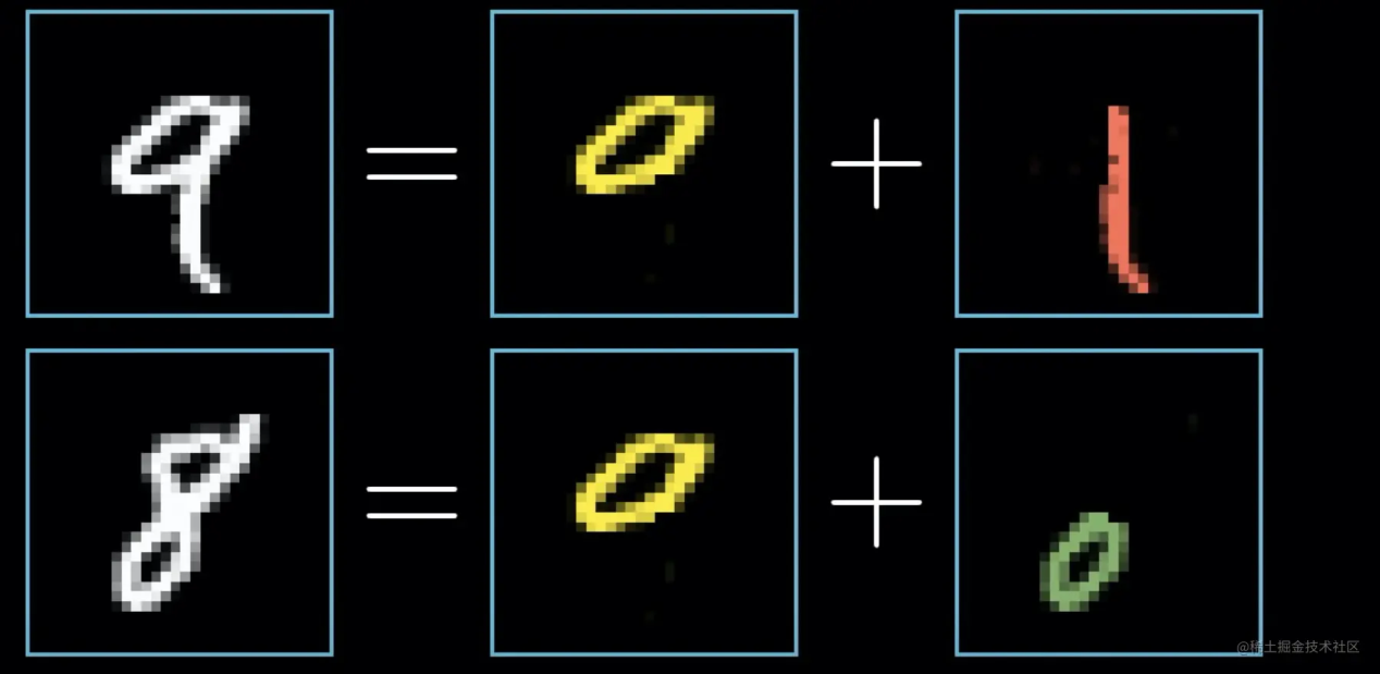
Their combination will give us results:
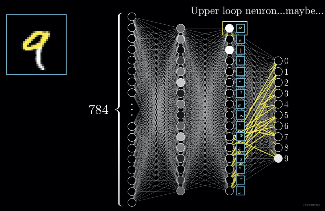
This is the third layer. We can determine that the second layer has a smaller granularity.
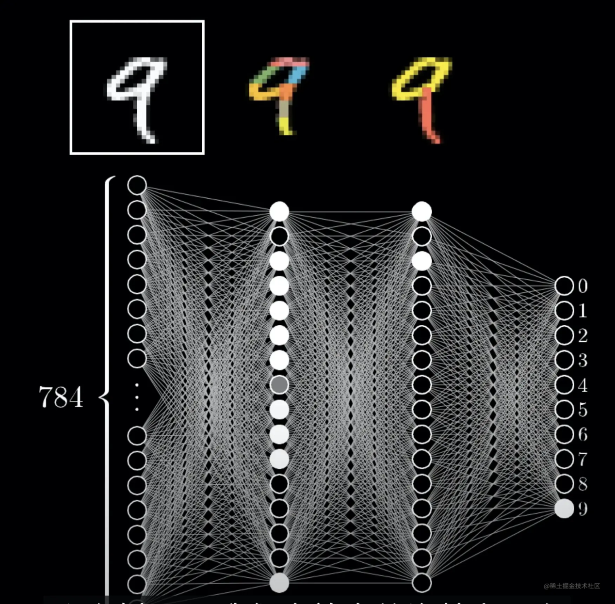
Here's the question. Does the real neural network work this way? It can be if the weight is set correctly. However, the model setting is much more complicated in practice. Here, we have simplified the model for easy understanding.
How can we achieve this effect? The answer lies in the weights, which refer to the lines of the neural network. Our activation values are obtained by calculating the values at the previous layer together with the weights.
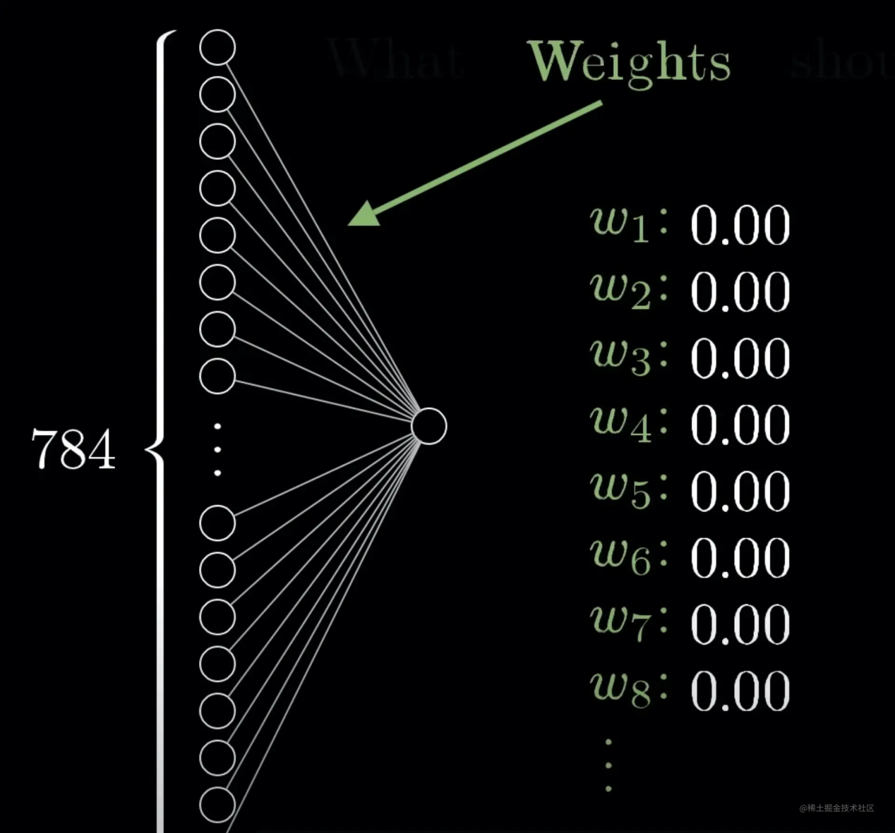
At first, our formula is a(L) = W * a(L-1). This means:
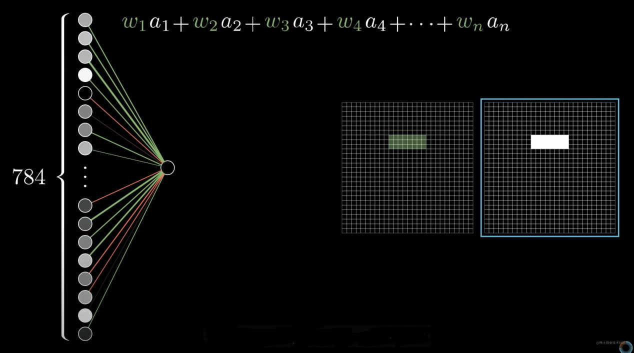
Therefore, if we want to recognize a horizontal line, we can just set the weight of the horizontal line pixels to 1 and the other to 0. We call the value above weighted value S.
As we said just now, this is the most basic formula. In practice, we often use an activation function to calculate the S value to ensure the activation value is within a certain controllable range.
Let's assume we need to control the value between zero and one. At this time, we can use an activation function called sigmoid, as shown in the following figure:
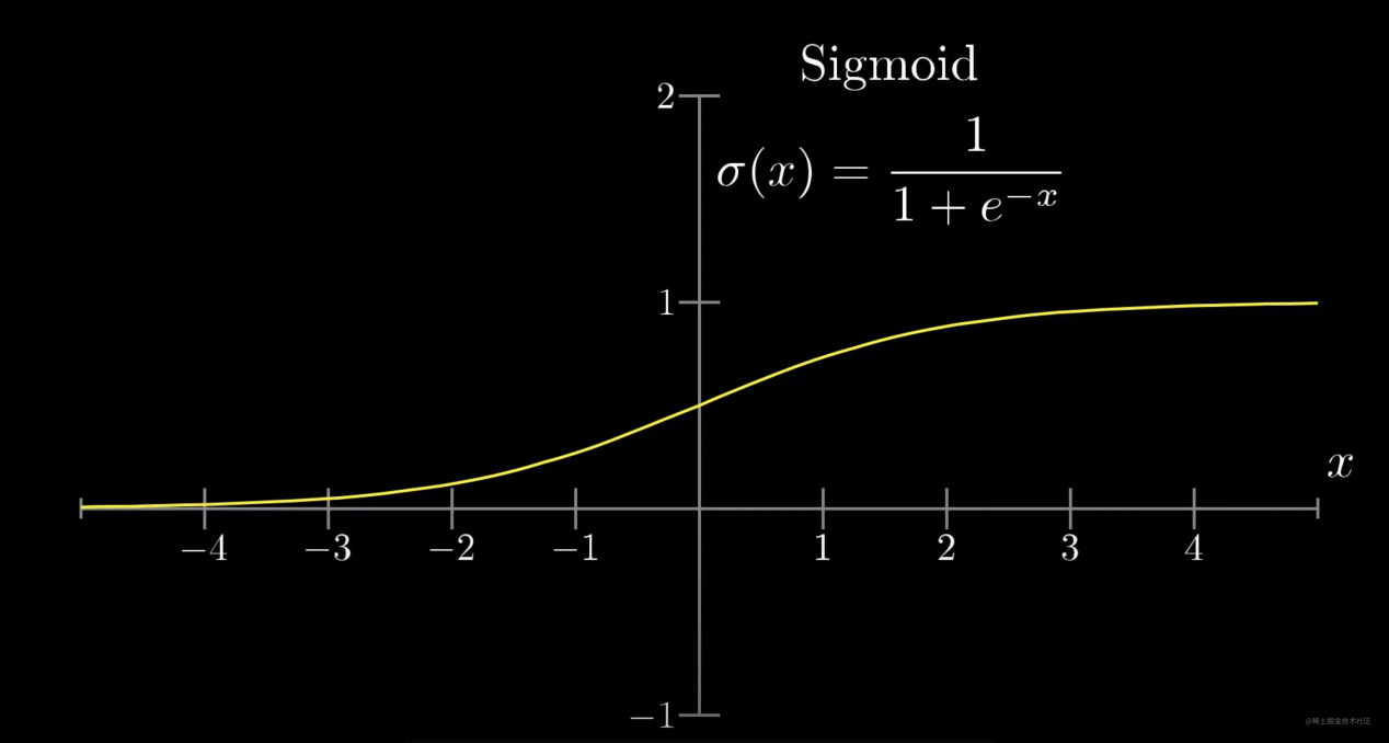
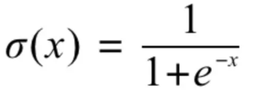
We have all learned this formula, whose value remains between zero and one. Let's find the formula for the activation value. The parameters involved include the weight:
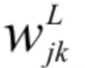
L indicates the number of deep layers, and j and k indicate the ordinal number of the activation values at the previous layer and the current layer, respectively. For the bias,

L represents the number of deep layers, and k represents the ordinal number of the activation value at this layer. We will calculate the weighted value S first:

We can get this formula:

Sometimes, if we want to light it up only when S is greater than 10 (light up if the final value is greater than 0.5), we need to add a bias value. Thus, this formula becomes:

b is the bias value. We can make some changes:

Finally, the formula becomes:

Well, we understand neural networks now. Here, we need to think about a question. How many bias values and weight parameters are needed?
The connection of the lines is in pairs, so there are 78416 + 1616 + 1610 weights in total. Bias values are required for each calculation of the next layer, so it is the sum of 16+16+10. The total is 78416 + 1616 + 1610 + 16+16+10 = 13002. A simple neural network requires so many parameters. Are you surprised?
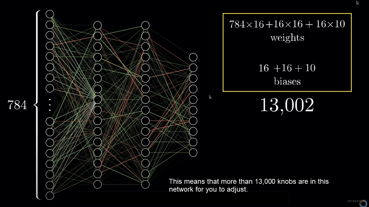
A well-trained neural network can recognize the picture correctly. A large number of complicated parameters are the prerequisite for strong adaptability.
Here, we understand the principle of forward propagation of neural networks.
However, it is still not enough. We said above that a well-trained network can recognize pictures correctly. Then, the question arises. How can we get a well-trained neural network?
The answer is a kind of self-regulation that uses the gradient descent algorithm to continue backpropagation.
Let's get back to the point. This kind of heavy workload is usually done by setting rules for the machine to adjust continuously. First of all, we need to be clear about the issues we need to focus on:
Let's take a look at the accuracy of the result first. It is simple. We can calculate the loss at the output layer:

a(n) represents the calculated value, and y(n) is the expected value. Here, we can get the loss value of the last layer. The greater the loss value, the further it is from the expectation.
When the cost is relatively large, how should we adjust? We must adjust a(n) to keep it close to the value of y(n). Do you still remember the formula for calculating a(n)? We can find that only the activation value a, weight w, and bias value b can be adjusted. The problem is that the activation value is also the a, w, and b at the previous layer, right? Then, we can only adjust w, b, and a at the first layer. a at the first layer is an input value, so we can ignore it. The key point is that we need to adjust all parameters, including the weight w and the bias value b.
Okay, we have a goal, right? The question is how to adjust these parameters. The answer is gradient descent.
Let's learn about gradient descent. First, recall Taylor's Formula:

Here, f′(x) is the gradient of the function f at x. The gradient of a one-dimensional function is a scalar (also called a derivative), as shown in the following figure:
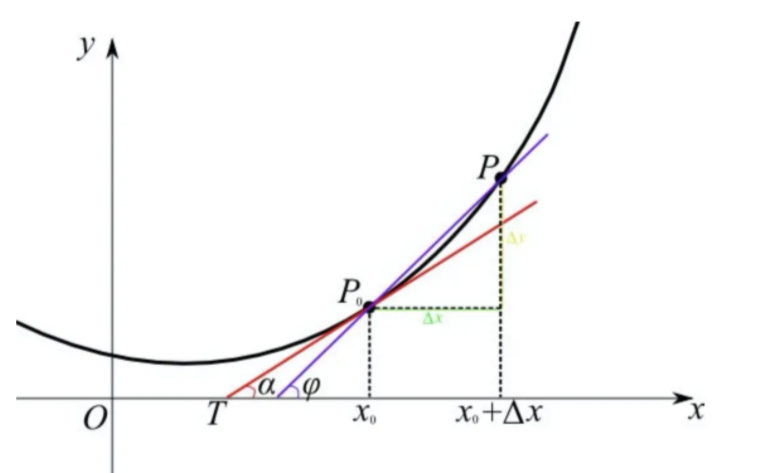
Next, find a constant η that is greater than 0 to ensure that ∣ηf′(x)∣ is small enough. Then, replace ϵ with −ηf′(x), and we will get:

If f′(x)≠ 0, then:

So:

This means we need to take the derivative of f(x) and set a positive number η small enough to make f(x) smaller. x-ηf(x) is the target value. This is the one-dimensional evaluation method.
Well, I believe many of you have already been clear by this time. Our goal is to reduce the loss, while loss C is obtained by all weights, bias values, and input values in each layer. So, we must get all ηf′(x) of weights and bias values to achieve the same goal. The process of getting all the vectors to be adjusted can be called:

Since we calculate backward layer by layer, it is called backpropagation.
First, calculate the adjustment amount of the output layer. Set the last layer as the L layer and the number of output layers to n.

This way, the error adjustment of the outermost layer is calculated. Then, calculate the second layer from the bottom: the L-1 layer. According to the chain rule:

Similarly, each adjustment difference of each layer needs to be calculated with the chain rule until the vector is obtained.

As to all adjustment vectors of w and b, do you remember what I mentioned earlier? There is a kind of self-regulation that uses the gradient descent algorithm to continue the backpropagation. The essence of the so-called model training is to continuously adjust parameters through backpropagation to get a suitable nonlinear combination. Thus, all samples can get the capability of ensuring that loss is in a reasonable range through this combination.
All complex tasks are left to machines, and humans only adjust them. This is particularly evident in model training.
The principle of neural networks has been shown here. Next, let's take a look at what a convolutional neural network is.
Convolutional neural networks are neural networks with special layers. It includes convolution layers, pooling layers, and full connection layers.

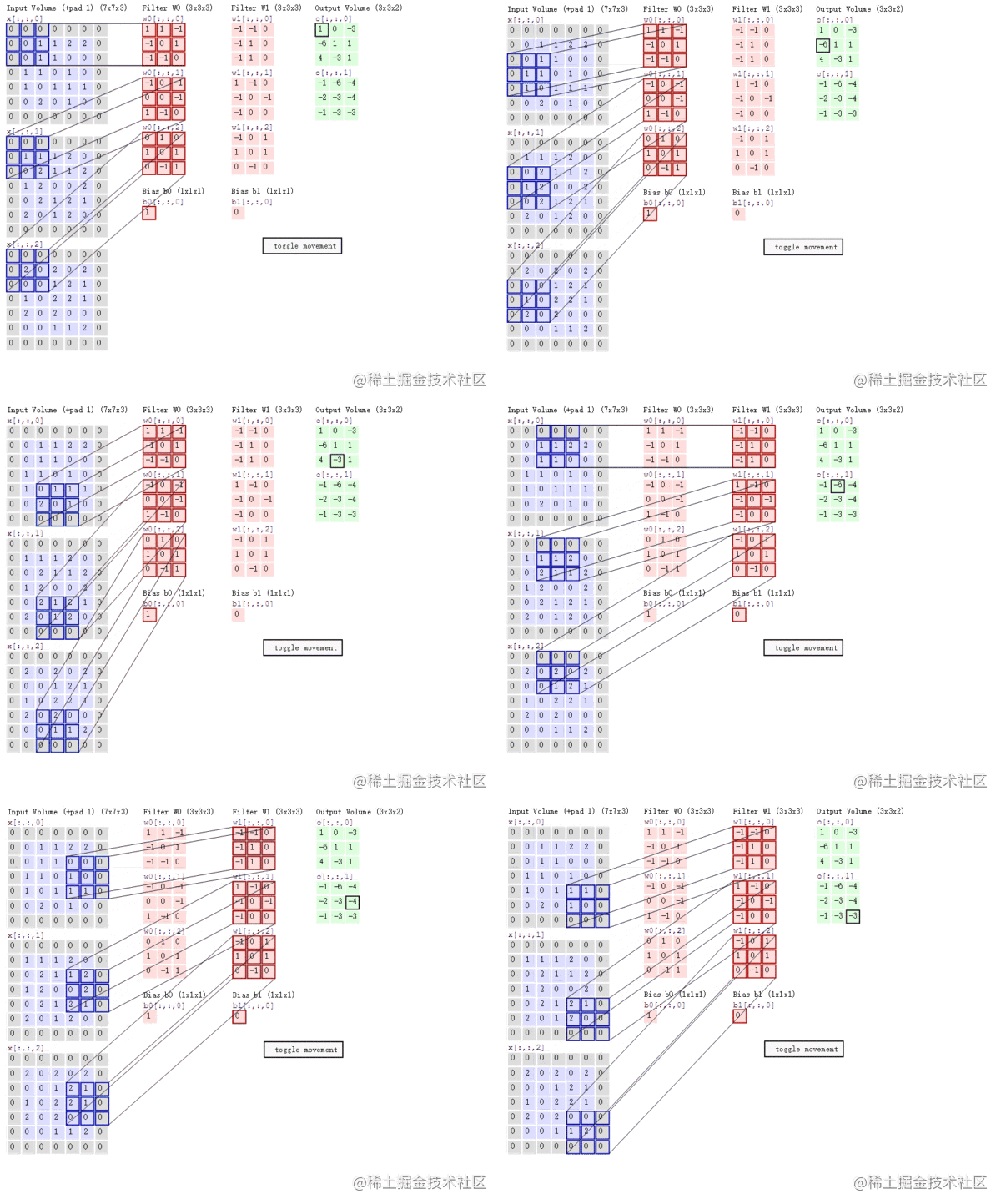
These layers have different functions. Let's take a look at the convolution layer first. The following figure shows the meaning of convolution:
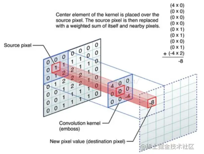
Essentially, multiple convolution kernels extract features of the original graph at the convolution layer. The convolution kernel is in the middle of the figure above. Compared with the processing of the weighted value S in the neural network part, it is not difficult to find that the convolution kernel can be regarded as a simple weight setting.
The parameters of the convolution layer include convolution kernel size, stride, and padding. They will be introduced below.
Feel the convolution kernel with a GIF image:
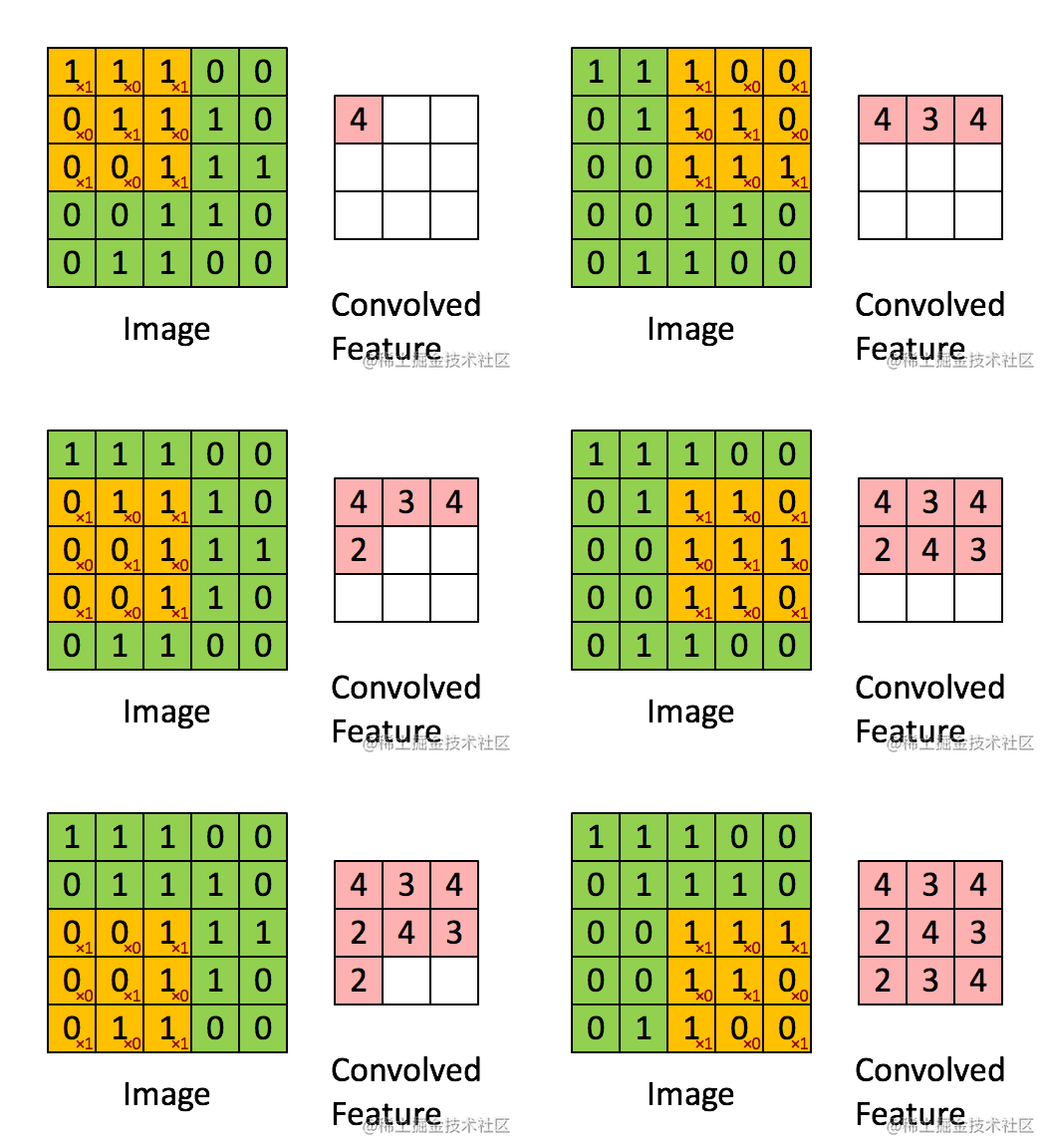
The convolution kernel here is sized 3*3, with each to be 1. In other words, all numbers are added up.
| 1 | 1 | 1 |
| 1 | 1 | 1 |
| 1 | 1 | 1 |
As shown above, some values are lost after the convolution of the input image and the convolution kernel. The edges of the input image are trimmed away. (Only some pixels are detected at the edges, and a lot of information there is lost.) This is because the pixels on the edge will never be in the center of the convolution kernel, and the convolution kernel cannot extend to the edge. This result is unacceptable to us. Sometimes, we even hope the input and output sizes should be consistent. You can pad the boundary of the original matrix before performing the convolution operation to solve this problem. It means you can fill some values on the boundary of the matrix to increase its size. Generally, 0 is used for padding.
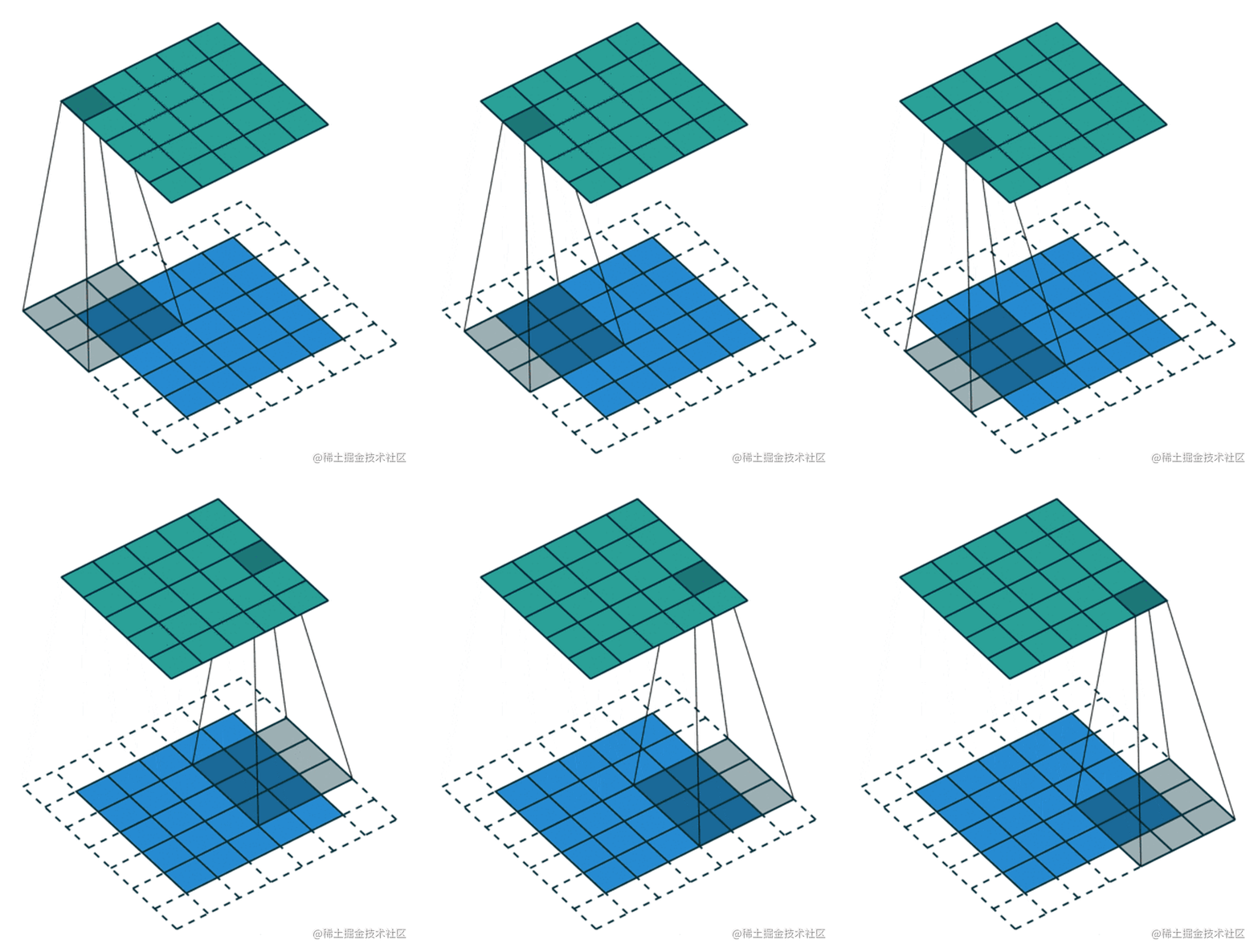
Padding is set to avoid information loss, and sometimes, we need to set the stride to compress the information. Please see the following image:
What does convolution do to the image, and why can it extract features? Let's take a look at a group of pictures:


The edge features are extracted by the commonly used convolution kernel called Laplace Operator. Then, the extracted edges are strengthened to get the sharpened pictures we commonly see.
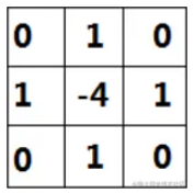
Laplace Operator
The effect of convolution kernels in different sizes differs, as shown in the following figure:


The picture in the lower part is much better. Now that we know the function of convolution kernels, let's move on to the pooling layer, which is also translated into the sampling layer. I prefer to call it the sampling layer because its main function is sampling. We can take a look at the process of max pooling to understand it better:
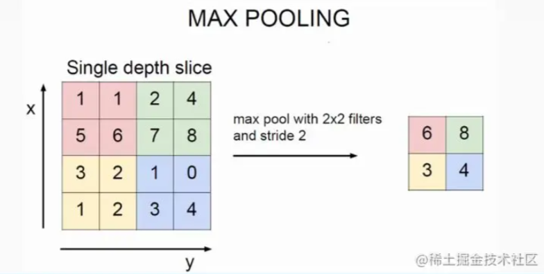
From the perspective of human understanding, it is to obtain the most obvious features. Why do we have to do this? We need to trace it back to history. This is because machines in the early stages did not have enough computing power, and this kind of sampling layer can significantly reduce computation. Another reason is to prevent overfitting.
The last layer is the full connection layer. The full connection layer does not need to be discussed anymore. It plays the role of classification. Its principle is virtually the same as the hidden layer mentioned earlier. The main function is abstraction and classification. It is worth noting that the last layer often contains the softmax activation function, which is good at classification.
So much for the introduction to the structure of convolutional neural networks! We need to remember that the structure we introduced here is a basic one, and many parts have been studied and optimized by many people. For example, the research achievements on convolution include tiled convolution, deconvolution, and dilated convolution. If you are interested, you can refer to related papers.
There are still some important concepts that need to be emphasized here:
Let's take a look at fine tune. An example will tell you what fine tune is. Let's suppose we need to train a linear model: y = x. If the weight given at the beginning is 0.1, it may take many steps of training to get a similar model.
However, if someone directly gives you a similar weight, the training is much faster, right? At this time, when you perform backpropagation, it is called fine tune. Of course, other people will not directly tell you the weight during real-life model training, but you can directly load other good models. Their parameters and weights have been verified well, so your training speed will be much faster. You can call this model the pre-training model and the process migration learning. The adjustment of parameters is called fine tune.
Fine tune has two advantages:
Speaking of imagenet, this is a very cool computer vision recognition project. It is currently the largest library of picture recognition in the world. It is established to simulate the human recognition system. The whole data set has about 15 million pictures and 22,000 categories. Surprisingly, they are annotated by humans, and the quality is ensured. Unfortunately, it does not include D2C. Otherwise, we can use it directly.
Please click the link below for more information: https://www.tensorflow.org/js/models
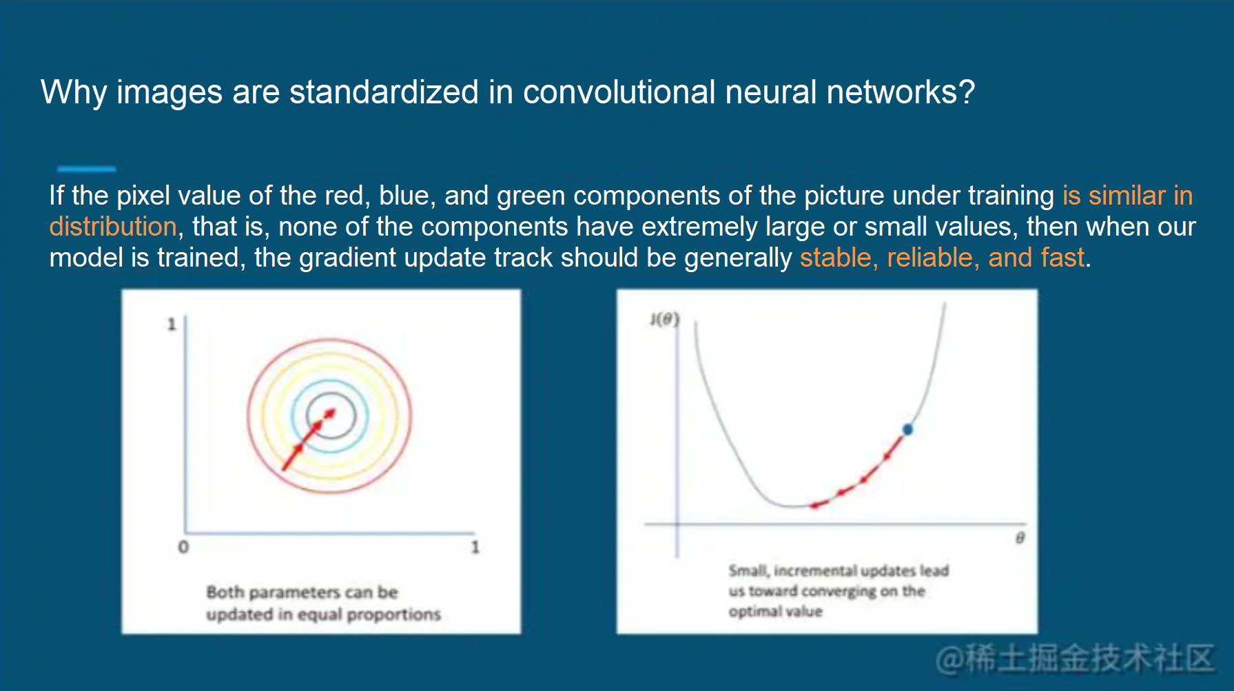
Image Standardization: Please see the pictures below for reference in this article.
Youku's Frontend Team Builds an Intelligent Material Generation Platform with imgcook

66 posts | 5 followers
FollowAlibaba Clouder - December 26, 2016
Alibaba Clouder - May 18, 2021
Alibaba Cloud MVP - July 9, 2021
Apache Flink Community - April 2, 2025
Alibaba Clouder - January 22, 2020
Alibaba Clouder - February 6, 2018

66 posts | 5 followers
Follow Container Compute Service (ACS)
A cloud computing service that provides container compute resources that comply with the container specifications of Kubernetes
Learn More Container Service for Kubernetes
Alibaba Cloud Container Service for Kubernetes is a fully managed cloud container management service that supports native Kubernetes and integrates with other Alibaba Cloud products.
Learn More Platform For AI
A platform that provides enterprise-level data modeling services based on machine learning algorithms to quickly meet your needs for data-driven operations.
Learn More Tongyi Qianwen (Qwen)
Top-performance foundation models from Alibaba Cloud
Learn MoreMore Posts by Alibaba F(x) Team