SLS Machine Learning Best Practices: Similarity Analysis for Time Series

This article introduces the best practices for time series similarity analysis, including time series clustering, similarity calculation, and correlation analysis.

Alibaba Cloud Log Service (SLS) provides a series of tools for DevOps and AIOps, which cover methods such as anomaly detection, time series clustering, and time series prediction. To make the service more accessible, we have integrated our algorithms into SQL to allow relevant configurations at the lowest cost. This article introduces the best practices for time series clustering and correlation analysis.

1) Scenarios

This article covers several useful functions for time series similarity analysis, involving time series clustering and similarity calculation using Log Service. These functions apply to the following scenarios:

When we have metrics data for n machines and want to quickly find out the CPU usage over a period of time to better understand the current system status.
When we specify a curve of a metric for a machine and want to know which machines have a similar curve for the specified metric.
When we manually input a time series curve (the access latency curve of a website) and want to determine which service has a similar curve for access latency changes in order to narrow down the troubleshooting scope.

The preceding scenarios come down to two aspects: time series clustering (by shape and by value) and determination of time series similarity.

2) Description

The SLS platform provides two functions. Check out the documentation page for more details.

ts_density_cluster
ts_hierarchical_cluster

The first function targets clustering based on the curve shape and its underlying core clustering algorithm is the algorithm of density-based clustering (DBSCAN). The second function targets clustering based on the similarity among original curves, with more emphasis on factors such as the Euclidean distance between curves. Its underlying core clustering algorithm is the hierarchical clustering algorithm. For more information about how these functions work, see my previous articles, or search for relevant information online. The following section describes how to use these functions in SLS.

3) Case Study

3.1) Data Exploration

query-01

* | select DISTINCT index_name, machine, region from log

query-02

* | select count(1) as num from (select DISTINCT index_name, machine, region from log)

query-03

* and index_name : load | 
select 
  __time__, 
  value, 
  concat(
    region, '#', machine, '#', index_name
  ) as ins 
from log order by __time__ 
limit 10000

query-04

* 
and index_name : load | 
select 
  date_trunc('minute', __time__) as time, 
  region, 
  avg(value) as value 
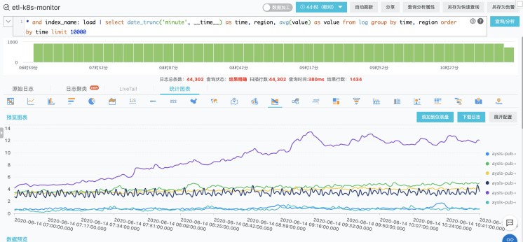
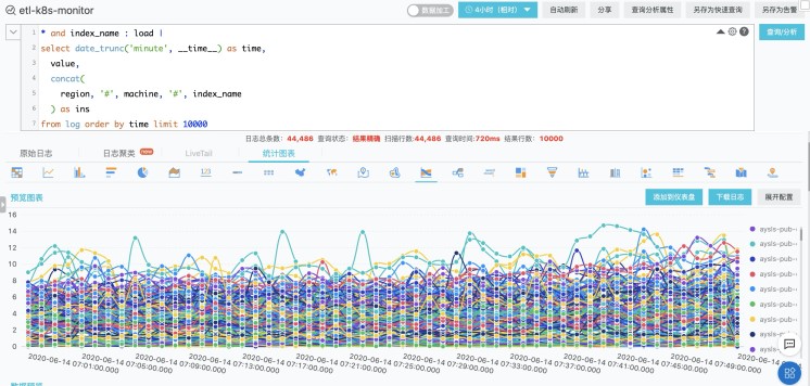
from log group by time, region order by time limit 1000

By executing query01, we get the following information, which indicates the number of different curves contained in the current Logstore and the identifier of each curve. To better observe the 1,300 curves, we use a flow diagram. However, charting all these curves in one diagram consumes considerable browser resources, and it would be very difficult to gain insight from the diagram even if it were generated. We use query04 to observe the visualization of a few curves and compare their visual effect with the effect of query03.

3.2) Clustering Practices

Based on the preceding observation, can we cluster some curves and group similar curves to reduce dimensions for visualized analysis?

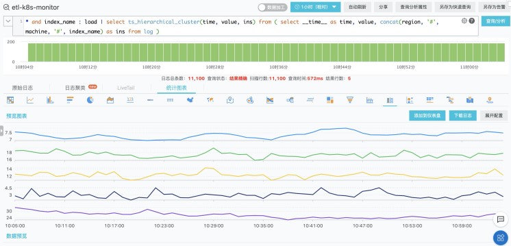
The following SQL statements enable quick curve clustering. In this example, the chosen metric is machine load because we want to know how usage changes for different machines. For this purpose, we use the ts_hierarchical_cluster function to get a facet chart. To make the chart more intuitive, store it in the dashboard.

* 
and index_name : load | 
select 
  ts_hierarchical_cluster(time, value, ins) 
from 
  (
    select 
      __time__ as time, 
      value, 
      concat(
        region, '#', machine, '#', index_name
      ) as ins 
    from 
      log
  )

3.3) Similarity Query

We get a list of machines that have a similar metric curve as aysls-pub-cn-beijing-k8s#192.168.7.254:9100#load by executing the following SQL statements and use the following flow diagram to visualize the result. The options for determining similarity offered by the similarity function include shape, manhattan, and euclidean.

* 
and index_name : load | 
select 
  cast(
    cast(ts_value as double) as bigint
  ) as ts_value, 
  cast(ds_value as double) as ds_value, 
  name 
from 
  (
    select 
      tt[1][1] as name, 
      tt[2] as ts, 
      tt[3] as ds 
    from 
      (
        select 
          ts_similar_instance(
            time, value, ins, 'aysls-pub-cn-beijing-k8s#192.168.7.254:9100#load', 
            10,
            'euclidean'
          ) as res 
        from 
          (
            select 
              __time__ as time, 
              value, 
              concat(
                region, '#', machine, '#', index_name
              ) as ins 
            from 
              log
          )
      ), 
      unnest(res) as t(tt)
  ), 
  unnest(ts) as t(ts_value), 
  unnest(ds) as t(ds_value) 
order by 
  ts_value 
limit 
  10000

Community

SLS Machine Learning Best Practices: Similarity Analysis for Time Series

1) Scenarios

2) Description

3) Case Study

3.1) Data Exploration

3.2) Clustering Practices

3.3) Similarity Query

悟冥

You may also like

Comments

悟冥

Related Products

Platform For AI

Simple Log Service

Epidemic Prediction Solution

DevOps Solution