×
Community Blog Kwai Builds Real-Time Data Warehouse Scenario-Based Practice on Flink

Kwai Builds Real-Time Data Warehouse Scenario-Based Practice on Flink

This article introduces the real-time data warehouse architecture built by Kwai based on Flink and offers solutions to some difficult problems.

This article is compiled from the topic entitled "Kwai Builds Real-Time Data Warehouse Scenario-Based Practice on Flink" shared by Li Tianshuo, an expert in Kwai Data Technology, during a Flink Meetup at Beijing Station on May 22. The contents include:

  1. Real-Time Computing Scenarios of Kwai
  2. Real-Time Data Warehouse Architecture and Safeguard Measures of Kwai
  3. Scenario Problems and Solutions of Kwai
  4. Future Planning

Visit the GitHub page. You are welcome to give it a like and stars!

1. Real-Time Computing Scenarios of Kwai

1

The real-time computing scenarios in Kwai business are divided into four main components:

  • Enterprise-Level Core Data: They include the market index, real-time core daily reports, and mobile data of the enterprise. The team will see the business market index of the enterprise, and each business line, such as video-related and live-related lines. Each of them will have a core real-time billboard.
  • Real-Time Metrics for Major Events: The core is real-time large-size screens. For example, the Kwai Spring Festival Gala event will use a large-sized overall screen to monitor every activity. A large-scale activity will be divided into N different modules, and we will have different real-time data billboards for each module.
  • Operation Data: Operation data mainly include two aspects: the creator and the content. On the operation side, creators and content want to see some information, such as the real-time status of the live rooms and the influence of the live rooms on the market index when launching a Big V event. Based on this scenario, we will collect multi-dimension data from various real-time large-size screens and some data from the market index.

It also includes the support of operational strategies. For example, we may discover some hot content, creators, and situations in real-time. We will output strategies based on these hot spots, which are also some support capabilities we need to provide.

Finally, it also includes the C-end data display. For example, Kwai has a creator center and an anchor center. There will be some closed broadcast pages, such as anchor closed broadcast. We also made some of the real-time data of closed broadcast pages.
  • Real-Time Features: They include search recommendation features and real-time advertising features.

2. Real-Time Data Warehouse Architecture and Safeguard Measures of Kwai

2.1 Objectives and Difficulties

2

2.1.1 Objectives

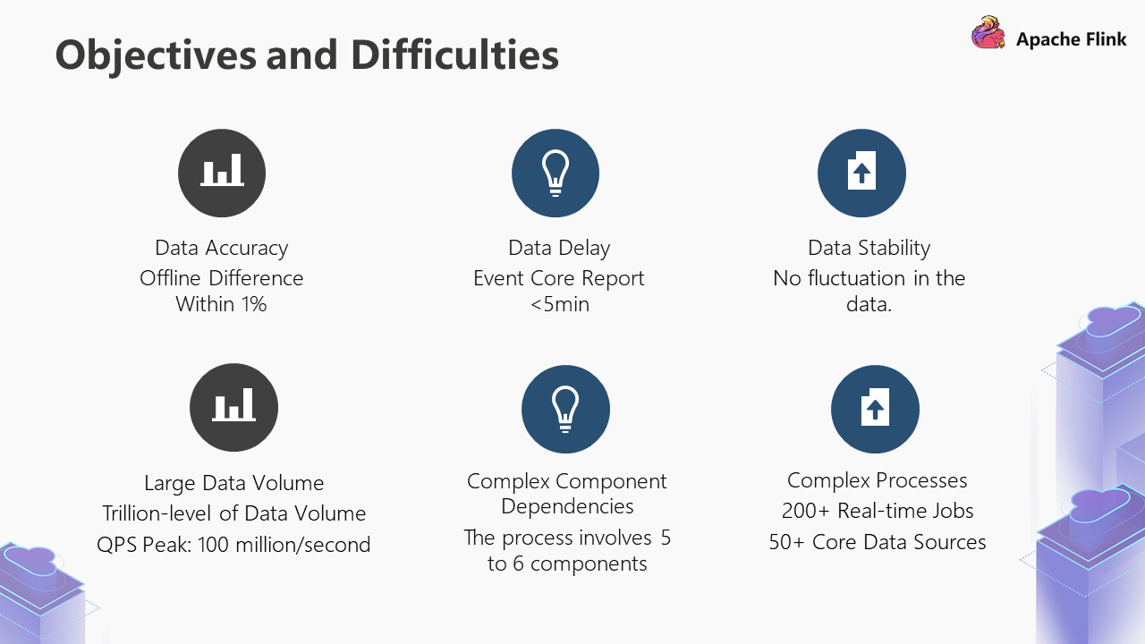
  • First of all, we are engaged in data warehouses, so we hope that all real-time metrics have corresponding offline metrics. The overall data difference between real-time metrics and offline metrics is required to be within 1%, which is the minimum standard.
  • The second is data delay. Its SLA standard is that the data delay of all core report scenarios during the activity cannot exceed five minutes, which includes the time after the job is hung up and the recovery time. If it exceeds the limit, the SLA is not up to standard.
  • The last one is about stability. In some scenarios, once a job restarts, the curve becomes normal, and it does not produce some obvious exceptions due to the job restart operation.

2.1.2 Difficulties

  • The first difficulty is the large amount of data. The overall daily ingress network traffic per day is at the trillions level. During the Spring Festival Gala, the peak QPS can reach 100 million per second.
  • The second difficulty is that component dependencies are more complex. Perhaps some of the processes depend on Kafka, some depend on Flink, and some depend on KV storage, RPC interface, and OLAP engine. We need to think about how to distribute in the processes so these components can work normally.
  • The third difficulty is that the links are complex. Currently, we have 200+ core business jobs and 50+ core data sources. The overall jobs exceed 1,000 pieces.

2.2 Real-Time Data Warehouse – Layered Model

Based on the three difficulties above, we will take a look at the data warehouse architecture on the image below:

3

As shown above:

  • Three different data sources are at the lowest level, including client log, server log, and Binlog log.
  • The public infrastructure layer is divided into two different layers. One is the DWD layer, which is responsible for detailed data, and the other is the DWS layer, which processes common aggregated data. DIM is what we call a dimension. A topic pre-layering is based on offline data warehouses. This topic pre-layering may include network traffic, users, devices, video production and consumption, risk control, and social networking.
  • The core work of the DWD layer is standardized cleaning.
  • The DWS layer associates dimension data with the DWD layer and generates some agglomerative layer with common granularity.
  • Further up is the application layer, including market index, multi-dimension analysis models, and business thematic data.
  • The scenario is at the top is.

The overall processes can be divided into three steps:

  • The first step is to conduct data-driven business, bringing in the business data.
  • The second step is to make data as assets, cleaning a lot of the data and forming some regular and orderly data.
  • The third step is business-driven data. Data will provide empowerment for business data value construction.

2.3 Real-Time Data Warehouse – Safeguard Measures

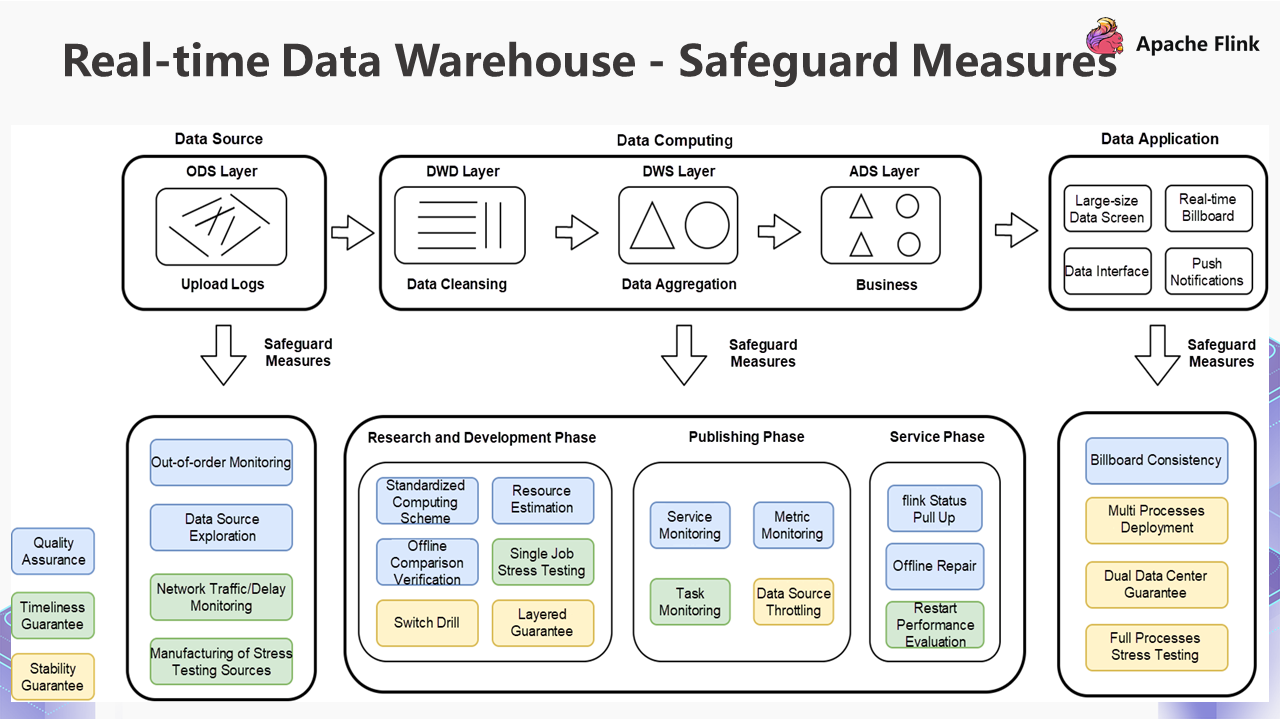
Based on the layer model above, we will take a look at the overall safeguard measures on the image below:
4

The guarantee layer is divided into three different parts: quality assurance, timeliness guarantee, and stability guarantee.

  • We will look at the quality assurance of the blue part first. For quality assurance, we have done out-of-order monitoring of data sources in the data source stage, which is based on our SDK collection, data sources, and offline consistency calibration. The computing process in the R&D phase is made up of three stages: the research and development phase, the online phase, and the service phase.

    • The research and development phase may provide a standardized model; some benchmarks exist based on this model. Then, we will perform offline comparison verification to ensure the quality is the same.
    • The online phase focuses on services monitoring and metrics monitoring.
    • In the services phase, if some exceptions occur, we will pull up the Flink status first. If some scenarios do not meet expectations, we will fix the overall offline data.
  • The second is the timeliness guarantee. For data sources, we also monitor the delay of data sources. There are two important things in the research and development stage:

    • The first thing is stress testing. Regular tasks will take the peak network traffic of the last 7-14 days to check if a task delay happened.
    • After passing the stress test, some tasks online and the restart performance evaluation will be carried out. It demonstrates the restart performance after CP recovery.
  • The last one is the stability guarantee, which will be used more in large-scale activities, such as switching drills and layered guarantee. We will perform throttling based on the previous stress testing results. The purpose is to ensure the job is still stable if it exceeds the limit. There will be no instability or CP failure. After that, we will have two different standards, one is a cold standby dual data center, and the other is a hot standby dual data center.

    • Cold Standby Dual Computer Room: When a single computer room is hung up, we will pull it up from another computer room.
    • Hot Standby Dual Data Centers: Deploy the same logic in each equipment room.

These are the overall safeguard measures.

3. Scenario Problems and Solutions of Kwai

3.1 PV/UV Standardization

3.1.1 Scenario

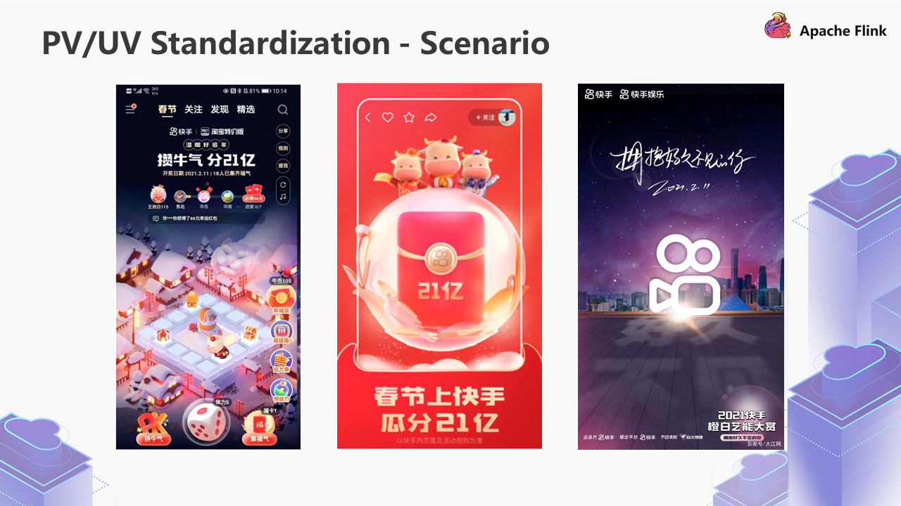
The first problem is PV/UV standardization. Take a look at the three screenshots below:
5

The first picture shows the warm-up scene of the Spring Festival Gala. This is a game page. The second and third pictures are the screenshots of the red envelopes sending activities and live room on the day of the Spring Festival Gala.

During the activity, we found that 60%-70% of the demands are to calculate the information on the page, such as:

  • How many people viewed this page, or how many people clicked this page?
  • How many people came to the activity altogether?
  • How many clicks did a pendant on the page get, and how many exposures did it generate?

3.1.2 Scheme

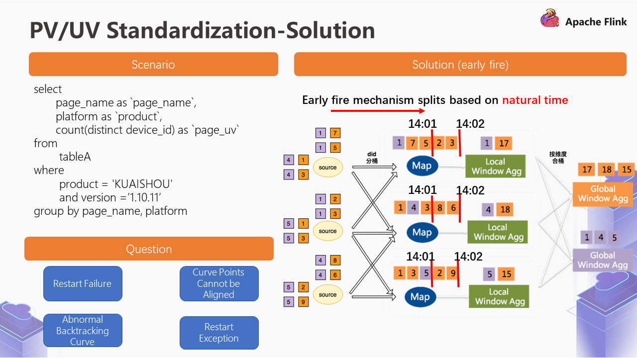
The following SQL represents the abstraction of this scenario:
6

Simply put, we filter conditions from a table, aggregate them according to the dimension level, and generate some Count or Sum operations.

Based on this scenario, the initial solution is shown on the right side of the figure above.

We adopted the Early Fire mechanism of Flink SQL to retrieve data from the Source data sources and then carry out the DID bucketing. For example, the purple part is divided into buckets according to this at the beginning. The reason for dividing buckets is to avoid hot spots problems of a certain DID. After bucketing, something called Local Window Agg will appear, adding the same type of data after the data bucketing. Local Window Agg is followed by the combined bucket of the Global Window Agg based on the dimensions. The concept of the combined bucket is to calculate the final results based on the dimensions. The Early Fire mechanism is to open a day-level window on the Local Window Agg and then output it to the outside every minute.

We encountered some problems in this process, as shown in the lower-left corner of the figure above.

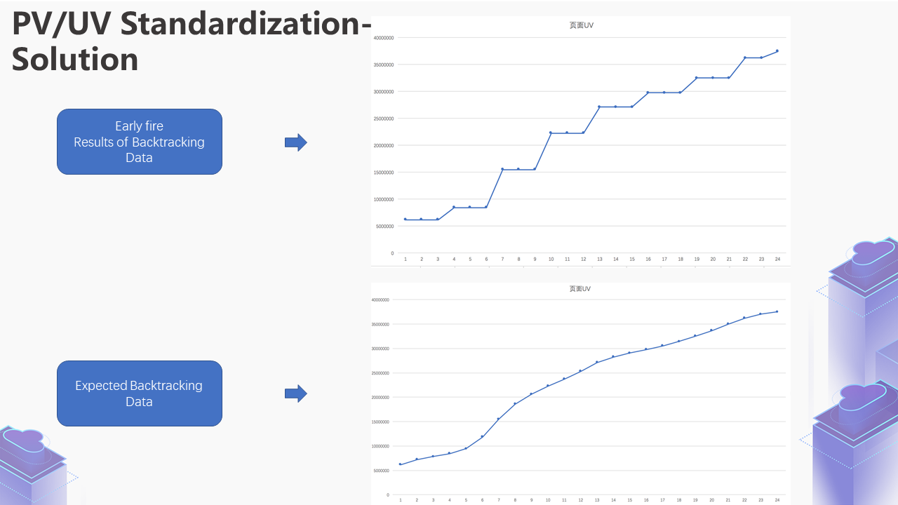
However, if there is a delay in the overall data or the backtracking history data (for example, Early Fire is performed once a minute), the data volume will be larger when the backtracking history is performed. This may lead to the data at 14:02 being read directly when the retroactive history is performed at 14:00, and the data at the time of 14:01 will be lost. What happens if the data are lost?
7

In this scenario, the curve at the top of the figure is the result of Early Fire backtracking historical data. The horizontal axis represents minutes, while the vertical axis represents the page UV up to the current moment. We found that some points are horizontal, meaning there is no data result. The curve depicts a steep increase. Then, it becomes a horizontal one. Later, it has another steep increase. The expected result of this curve is the smooth curve at the bottom of the figure.

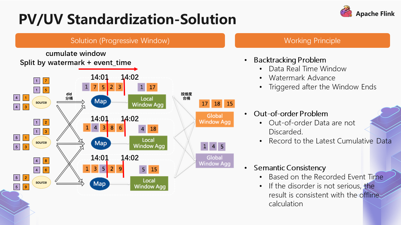
We used the Cumulate Window solution to solve this problem, which is also involved in Flink 1.13 version, and its principle is the same.
8

The data opens a large day-level window, and a small minute-level window is opened under the large one. The data falls to the minute-level window according to the Row Time:

  • Watermark advances the event_time of the window, and it will be triggered once. This way, the problem of backtracking can be solved. The data fall on the real window, and Watermark advances, which will be triggered after the window ends.
  • In addition, this method can solve the problem of disorder to a certain extent. For example, its out-of-order data is a state that is not discarded and will record the latest accumulated data.
  • Finally, it is about semantic consistency, which will be based on event time. If the disorder situation is not serious, the consistency with the batch processing results is quite high.

The section above is a standardized solution for PV/UV.

3.2 DAU Compute

3.2.1 Background

The following section introduces the DAU compute:
9

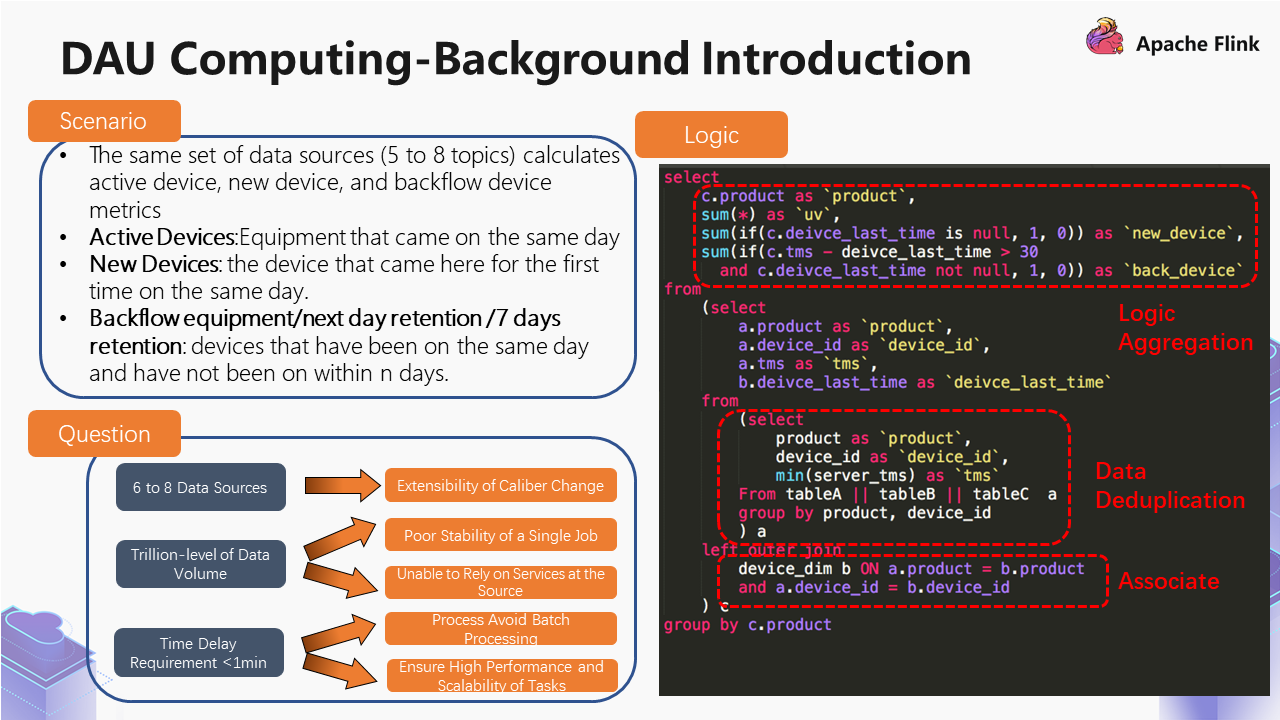
We monitored active devices, new devices, and backflow devices across the market index:

  • Active devices refer to devices that come on the same day.
  • New devices refer to devices that have been here that day and have not been here before that day.
  • Backflow devices refer to devices that have been here on the same day and have not been here within N days.

However, we may need 5-8 different topics to calculate these metrics.

We will take a look at how logic be calculated in the offline process.

First of all, we calculate the active devices, merge them, and do the day-level deduplication under a dimension. Then, we associate the dimension table, which includes the first and last time of the device. It refers to the time of the first and last access of the devices up to yesterday.

Once we get the information, we can perform logical computing. Then, we will find that the new devices and backflow devices are sub-tags in the active devices. The new devices will perform logical processing, and the backflow devices will perform logical processing for 30 days. Based on this solution, can we write a SQL to solve this problem?

We did this at the beginning, but we encountered some problems:

  • The first problem: We have 6-8 data resources, and the caliber of the market index is often fine-tuned. If it is a single job, it must be changed during the process of each fine-tuning, and the stability of the single job will be poor.
  • The second problem: The amount of data is at the trillions level, which will lead to two situations. The stability of a single job of this magnitude is poor, and the KV storage used when associating dimension tables is in real-time. Such an RPC service interface cannot guarantee service stability in the scenario of the trillions level of data.
  • The third problem: People have high requirements for the delay, which must be less than one minute. Batch processing should be avoided for the entire process. If a single point failure of task performance happens, we must ensure high performance and scalability.

3.2.2 Technical Protocols

In view of the problems above, we will next explain how to solve them below:
10

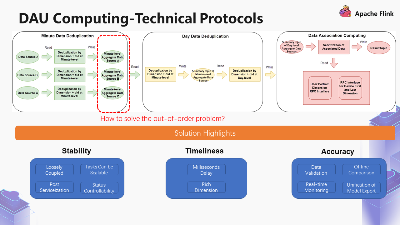
As shown in the example above, the first step is to deduplicate the three data sources (A B C) at the minute level according to the dimension and DID. After deduplication, three data sources at the minute level are obtained. Then, they are unionized together, and the same logical operations are performed.

The entry of the data sources changes from the trillions level to the tens of billions level. After the minute level is deduplicated, the generated data sources can change from the tens of billions level to the billions level.

In the case of the billions level of data, we will associate data servitization, which is a more feasible scheme. It associates the RPC interface of the user portrait. After obtaining the RPC interface, it is finally written into the target topic. This target topic will be imported into the OLAP engine to provide multiple different services, including mobile version service, large-size screen service, and metrics billboard service.

This scheme has three advantages, including stability, timeliness, and accuracy.

  • Stability: Loose coupling means when the logic of data source A and the logic of data source B need to be modified, they can be modified separately. The task also can be scaled out. Since we split all the logic into fine granularity, when network traffic problems occur in some places, it will not affect the following parts. As a result, it is easy to scale out. In addition, it has the advantages of service-oriented posting and state controllability.
  • Timeliness: We achieve a millisecond delay and have a wide range of dimensions. Overall, 20+ dimensions are for multi-dimensional aggregation.
  • Accuracy: We support data verification, real-time monitoring, and unification of model export.

In this case, we encountered another problem-disorder. For the three different jobs above, there will be a delay of at least two minutes for each job to restart. The delay will cause the downstream data sources to be unconnected.

3.2.3 Delay Computing Scheme

What could we do if we encounter the disorder above?
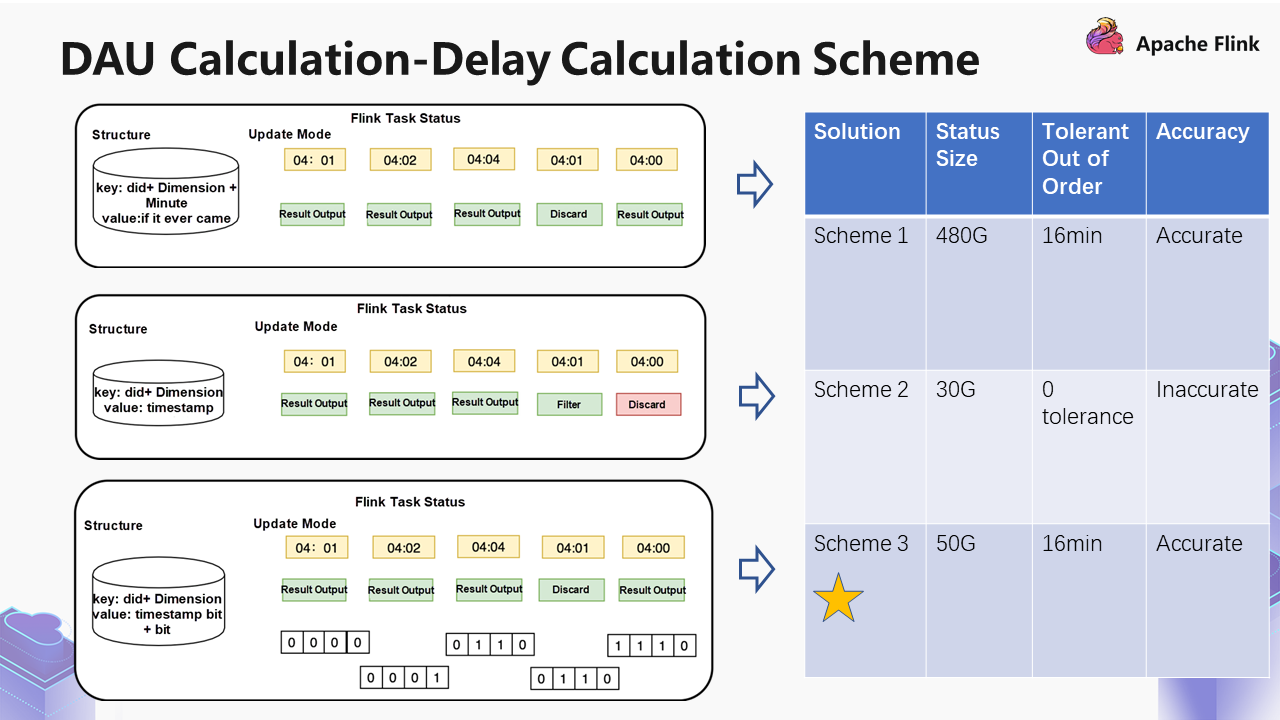
11

We have three solutions:

  • The first solution is to use "DID + dimension + minutes" for deduplication and set the Value to "have been here or not." For example, if one comes from the same DID at 04:01, it will output the result. Similarly, 04:02 and 04:04 will also output the results. However, if it comes again at 04:01, it will be discarded. If it comes at 04:00, the result will still be output.

Some problems will occur with this solution. Since we save it by minute, the size of the status of saving 20 minutes is twice the size of saving 10 minutes. Later, the size of this status is uncontrollable; therefore, we changed to solution 2.

  • In the second solution, the approach would involve a hypothetical premise, which implies there is no data source disorder. In this case, the key stores "DID + dimension" and the Value is "timestamp." Its update method is shown in the figure above.

At 04:01, a piece of data comes, and the result is output. At 04:02, a piece of data comes. If it is the same DID, it will update the timestamp and still carry out the result output. 04:04 follows the same logic, and it updates the timestamp to 04:04. If a piece of 04:01 data comes later, it finds that the timestamp has been updated to 04:04, and it will discard this data.

This approach reduces some of the required statuses by itself, but there is zero tolerance for disorder. Since we are not good at solving this problem, we have come up with solution 3.

  • Solution 3 is based on the timestamp of solution 2, adding a ring-like buffer and allowing disorder within the buffer.

For example, a piece of data comes at 04:01, and the result is output. When a piece of data comes at 04:02, it will update the timestamp to 04:02 and record that the same device came at 04:01. If there is another piece of data at 04:04, it will make a displacement according to the corresponding time difference through this logic to ensure that it can tolerate a certain amount of disorder.

Take a look at these three solutions below:
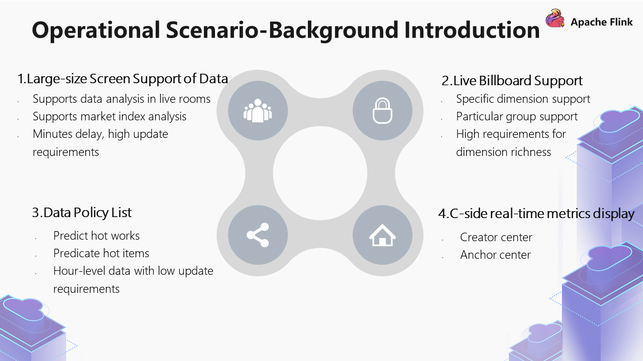
  • Solution 1: The status size of a single job is about 480G when 16 minutes of disorder is tolerated. Although this approach ensures accuracy, the recovery and stability of the operation are completely uncontrollable, so we still give up this solution.
  • Solution 2 has a status size of about 30G, which is zero tolerant of disorder. However, the data is inaccurate. Since we have high requirements for accuracy, we also abandoned this solution.
  • Compared with solution 1, the status of solution 3 has changed but not increased much, and the overall effect can be achieved with solution 1. The tolerance time for disorder in solution 3 is 16 minutes. If we update a job normally, 10 minutes is enough time to restart it, so we finally chose solution 3.

3.3 Operation Scenarios

3.3.1 Background

12

The operation scenarios can be divided into four parts:

  • The first is large-size screen support of data, including analysis data of a single live room and market index. It requires minute-level delay and has high update demands.
  • The second is the live billboard support. The data of the live billboard will be analyzed in specific dimensions and supported by particular groups. The requirements for dimension richness are high.
  • The third is the data strategy list, which mainly predicts popular works and items. It requires hourly data and has relatively low update requirements.
  • The fourth is the real-time metrics display on the C side. The query volume is large, but the query mode is fixed.

The following is an analysis of the different scenarios generated by these four different statuses.
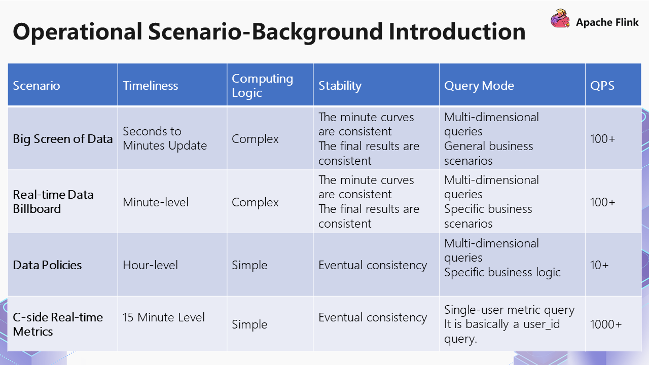
13

There is virtually no difference among the first three types except for the query mode. Some are specific business scenarios, and some are general business scenarios.

The third and fourth types have low requirements for update and high requirements for throughput, but the curves in the processes do not require consistency. The fourth query mode is more of a single entity query, querying what metrics will be used. The QPS requirements are high.

3.3.2 Technical Protocols

What could we do for the four different scenarios above?
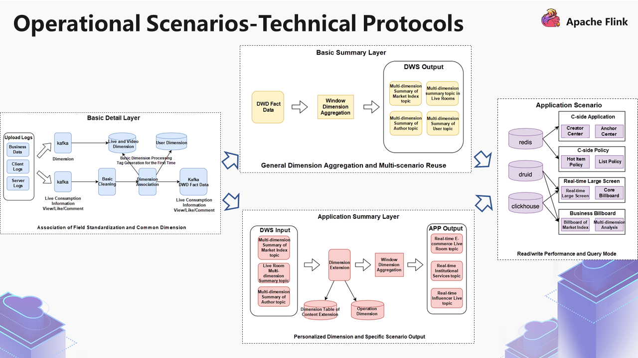
14

  • First, we will look at the basic detail layer (left in the figure above.) The data source has two processes, one is the consumption stream, such as the consumption information of livestreaming, and the view, like, and comment. After a round of basic cleaning, we will conduct dimension management. The upstream dimension information comes from Kafka. Kafka writes some content dimensions and puts them into KV storage, including some user dimensions.

After these dimensions are associated, they are finally written to the DWD fact layer of Kafka. We have performed the operation of Level 2 cache to improve performance.

  • At the top of the figure above, we read the data of the DWD layer and summarized it. The core is to aggregate the window dimension to generate four kinds of data with different granularity, including the multi-dimension summary topic of the market index, the multi-dimension summary topic of the live room, the multi-dimension summary topic of authors, and the multi-dimension summary topic of users. These are all data of common dimensions.
  • At the bottom of the figure above, based on these common dimension data, we will process the personalized dimension data, which is in the ADS layer. After receiving these data, there will be dimension expansion, including content expansion and operation dimension expansion. Then, we perform aggregation, such as e-commerce real-time topic, organization services real-time topic, and Big V live real-time topic.

Dividing into these two processes would have one benefit: One place deals with the general dimension, and the other deals with the personalized dimension. The requirements for the general dimension guarantee will be higher, while the personalized dimension will carry out a lot of personalized logic. If these two are coupled together, exceptions will occur often during the task. The responsibilities of each task are not clear, and such a stable layer cannot be constructed.

  • In the picture above (on the right), we used three different engines. Simply put, Redis query uses the C side scenario, and OLAP query uses the scenarios of large-size screens and business billboards.

4. Future Planning

Three scenarios were introduced above. The first scenario is the computing of standardized PU/UV, the second scenario is the overall solution of DAU, and the third scenario is how to solve the problems on the operation side. We have some future plans based on this content, which are divided into 4 parts.
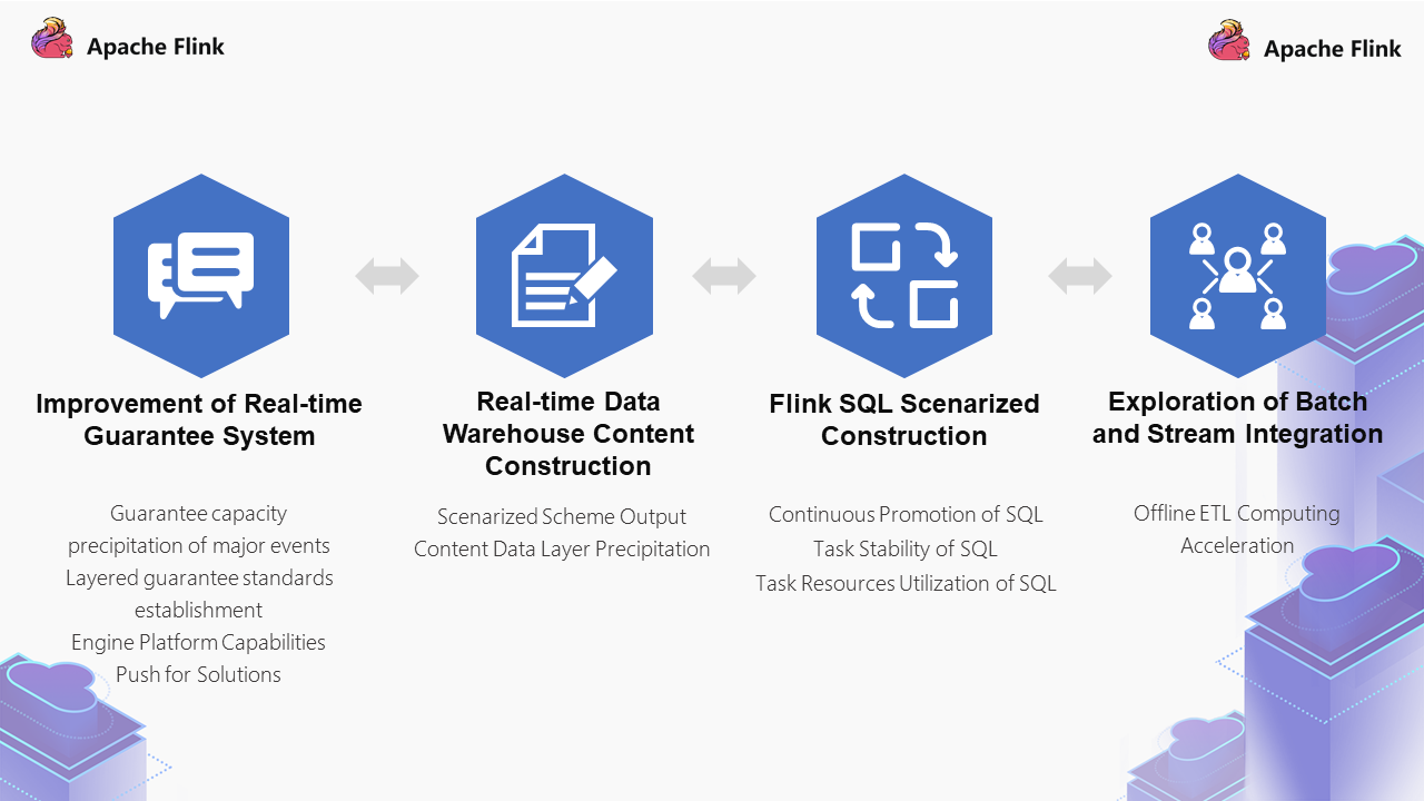
15

The first part is the improvement of the real-time guarantee system:

  • On the one hand, we will launch some large-scale activities, including the Spring Festival Gala and subsequent normalization activities. In view of the guarantee of these activities, we have a set of norms for platform construction.
  • The second is to set the standards of layered guarantee. There will be a standardized interpretation stating which operations are of what kind of guarantee level/standard.
  • The third is to promote the solution of engine platform capabilities, including some engines of Flink tasks. There will be a platform based on the engines. We will perform specifications based on this platform, the standardization of the promotion.

The second part is the real-time data warehouse content construction:

  • On the one hand, it is the output of a scenario-based solution. For example, there will be some general solutions for activities, instead of developing a new solution for each activity.
  • On the other hand, it is the content data layer precipitation, such as the current data content construction. There are some missing scenarios in terms of thickness, including how the content can better serve the upstream scenarios.
  • The third part is the scenarized construction of Flink SQL, including continuous promotion of SQL, task stability of SQL, and task resource utilization of SQL. In the process of estimating resources, we will consider what kind of solution SQL will use in what QPS scenario and what situation it can support. Flink SQL can reduce labor efficiency significantly, but in this process, we want to make business operations easier.
  • The fourth part is the exploration of batch and stream integration. The real-time data warehouse scenario will perform offline ETL computing acceleration. We will have many hour-level tasks. For these tasks, some logic in batch processing can be put into stream processing to get solved, which is a great improvement for the SLA system of the offline data warehouse.
0 1 0
Share on

Apache Flink Community

132 posts | 41 followers

You may also like

Comments

Apache Flink Community

132 posts | 41 followers

Related Products