Application of Deep Reinforcement Learning in Time Series Data Compression - ICDE 2020 Paper

This article provides an in depth overview of the research, results, and exploration conducted on data compression using deep reinforcement learning by Alibaba.

By Xinyang

Acknowledgment of the People Involved

During the composition of this paper, Yanqing Peng, Feidao, Wangsheng, Leyu, Maijun, and Yuexie contributed a lot. Here, I want to show my special appreciation to Feidao's guidance and help. I also want to express gratitude for Xili's support and Deshi's help and support.

Preface

"There are gaps between cow bones, while a knife is extremely thin. Therefore, it is easy to cut the bones with the knife." - Abstracted from Pao Ding Jie Niu.

This Chinese saying means that you can do a job well as long as you understand the rules for doing it.

With the application and popularization of the mobile Internet, Internet of Things (IoT), and 5G, we are stepping into the age of the digital economy. The resulting massive data will be an objective existence and will play an increasingly important role in the future. Time series data is an important part of massive data. In addition to data mining, analysis, and prediction, how to effectively compress the data for storage is also an important topic of discussion. Today, we are also in the artificial intelligence (AI) age, where deep learning has been widely used. How can we use it in more applications? The essence of deep learning is to make decisions. When we use deep learning to solve a specific problem, it is important to find a breakthrough point and create an appropriate model. On this basis, we can sort out data, optimize the loss, and finally solve the problem. In the past, we conducted some research and exploration in data compression by using deep reinforcement learning and found some results. We published a paper titled "Two-level Data Compression Using Machine Learning in Time Series Database" in ICDE 2020 Research Track and made an oral report. This article introduces our research and exploration, and we hope that you will find it helpful for other scenarios, at least for the compression of other data.

1. Background

1.1 Time Series Data

As its name implies, time series data refers to data related to time series. It is a common form of data. The following figure shows three examples of time series data: a) electrocardiogram, b) stock index, and c) specific stock exchange data.

From the view of users, a time series database provides query, analysis, and prediction of massive data. However, at the underlying layer, the time series database must perform massive operations, including read and write, compression and decompression, and aggregation. These operations are performed on the basic unit of time series data. Generally, time series data is described by two 8-byte values in a unified manner, which can also be simplified.

As you can imagine, electronic devices generate massive time series data of different types every day, which requires huge storage space. In this case, compressing the data for storage and processing is something natural. Then, the point is how to more efficiently compress the data.

1.2 Reinforcement Learning

Depending on whether samples have groundTruth, machine learning is classified into supervised learning, unsupervised learning, and reinforcement learning. As the name implies, reinforcement learning requires continuous learning, which does not require groundTruth. In the real world, groundTruth is also often unavailable. For example, human cognition is mostly a process of continuous learning in iterative mode. In this sense, reinforcement learning is a process and method that is more suitable or popular for dealing with real-world problems. So, many people say if deep learning gradually becomes a basic tool for solving specific problems like C, Python, and Java, reinforcement learning will be a basic tool of deep learning.

The following figure shows the classic schematic diagram of reinforcement learning, with the basic elements of state, action, and environment. The basic process is: The environment provides a state. The agent makes a decision on an action based on the state. The action works in the environment to generate a new state and reward. The reward is used to guide the agent to make a better decision on an action. The cycle works repeatedly.

In comparison, the common supervised learning, which can be considered special reinforcement learning, is much simpler. Supervised learning has a definite target, groundTruth. Therefore, the corresponding reward is also definite.

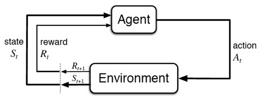
Reinforcement learning can be classified into the following types:

Deep Q Network (DQN): This type is more in line with people's intuitive feeling logic. It trains a network that is used to evaluate the Q-value and can provide rewards corresponding to actions based on any state. Then, it selects the action with the largest reward. During the training, DQN evaluates the results of the "estimated Q-value" and "real Q-value" for backpropagation. In this way, the network can evaluate the Q-value more accurately.
Policy Gradient: This type is more end-to-end. It trains a network to directly output a final action for any state. DQN requires that the Q-values of continuous states also be continuous, which does not apply to cases like chess playing. Policy Gradient ignores the internal process and directly outputs actions, which is more universal. However, Policy Gradient makes evaluation and convergence more difficult. The general training process is: Policy Gradient takes multiple actions at random for a state, and evaluates the results of all the actions for backpropagation. Finally, the network outputs a better action.
Actor-Critic: This type combines the first two types for complementation. On the one hand, it uses the Policy Gradient network to output actions for any state. On the other hand, it uses DQN to quantitatively evaluate the actions output by Policy Gradient and uses the result to guide the update of Policy Gradient. As its name implies, Actor-Critic demonstrates a relationship similar to the relationship between an actor and a critic. During the training, the Actor (Policy Gradient) network and the Critic (DQN) network are trained at the same time. The training of "Actor" only needs to follow guidance from "Critic." Actor-Critic has many variants and is also a major branch of current DRL theoretical research.

2. Compression of Time Series Data

Undoubtedly, in the real world, it is necessary to compress massive time series data. Therefore, the academic and industrial worlds have done a lot of research, including:

Snappy: compresses integers or strings. It uses long-distance prediction, run-length encoding (RLE), and has many applications, including InfuxDB.
Simple8b: performs delta processing for data. If all deltas in the resulting deltaValues are the same, RLE encoding is applied to them. If the deltas are different, numbers 1 to 240 (the bits of each number according to the code table) are packed into data in the unit of 8 bytes based on the code table that contains 16 entries. Simple8b has many applications, including InfuxDB.
Compression Planner: introduces some general compression tools, such as scale, delta, dictionary, huffman, run length, and patched constant. Then, it proposes to statically or dynamically combine these tools to compress data. This idea is novel, but the performance is not proven.
ModelarDB: focuses on lossy compression based on the tolerable loss specified by a user. The basic idea is to maintain a small buff and detect whether data conforms to a certain pattern (straight-line fitting of a slope.) If it fails, switch the pattern and start a new buff. ModelarDB applies to the lossy IoT field.
Sprintz: also applies to the IoT and focuses on the processing of 8- or 16-bit integers. It uses scale to perform prediction and uses RLC to encode the resulting deltas and conduct bit-level packing.
MO: is similar to Gorilla but excludes bit-packing. In this method, all data operations are byte-aligned, which lowers the compression ratio but improves the processing performance.
Gorilla: is the compression algorithm that is used for the sofa in the Facebook high-throughput real-time system. It is used for lossless compression and widely used in various fields, such as the IoT and cloud services. Gorilla introduces delta-of-delta to process timestamps, runs xor to convert data, and then uses Huffman for encoding and bit-packing. The following figure shows the schematic diagram of Gorilla.

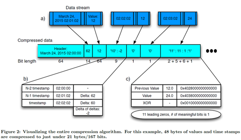
There are also many related compression algorithms. In general,

They use single modes or limited static modes to compress data.
To increase the compression ratio, many compression algorithms use bit-packing or lossy compression. However, they are not friendly to the increasingly popular parallel computing.

3. Two-Stage Compression Algorithms Based on Deep Learning

3.1 Characteristics of Time Series Data Compression

Time series data comes from different fields, such as the IoT, finance, Internet, business management, and monitoring. Therefore, they have different forms and characteristics, and also have different requirements for data accuracy. If only one unified compression algorithm can be used for non-differential processing, this algorithm should be a lossless algorithm that describes data in the unit of 8 bytes.

The following figure shows some examples of time series data used in Alibaba Cloud business. Regardless of the macro or micro view, there are various data patterns, both different in shape curve and data accuracy. Therefore, compression algorithms must support as many compression patterns as possible, so an effective and economic compression pattern can be selected for compression.

A large-scale commercial compression algorithm for time series data must have three important characteristics:

Time correlation: Time series data is strongly time-correlated, and corresponding data is almost continuous. The sampling interval is often 1 second or 100 milliseconds.
Pattern diversity: As shown in the preceding figure, the patterns and characteristics are largely different.
Data massiveness: Massive data needs to be processed every day, every hour, and every second. The total data volume processed every day is around10-PB. Therefore, compression algorithms must be highly efficient and have a high throughput.

3.2 Core Concepts of New Algorithms

The essence of data compression can be divided into two stages. The first stage is transformation, at which data is transformed from one space to another space with a more regular arrangement. The second stage is delta encoding, at which various methods can be used to identify the resulting deltas after delta processing.

Based on the characteristics of time series data, we can define the following six basic transforming primitives. All of them are expandable.

Then, we can define the following three basic differential coding primitives. All of them are also expandable.)

Next, should we sort and combine the preceding two tools for compression? This is feasible, but the effect is not good, because the cost proportion of pattern selection and related parameters are too high. The control information of 2 bytes (primitive choice + primitive parameter) accounts for 25% of data to be expressed in 8 bytes.

Therefore, a better solution is to express the data characteristics at abstracted layers, as shown in the following figure. Create a control parameter set to better express all situations. Then, select proper parameters at the global (timeline) level to determine a search space, which contains only a small number of compression patterns, such as four patterns. During the compression of each point in the timeline, traverse all the compression patterns and select the best one for compression. In this solution, the proportion of control information is about 3%.

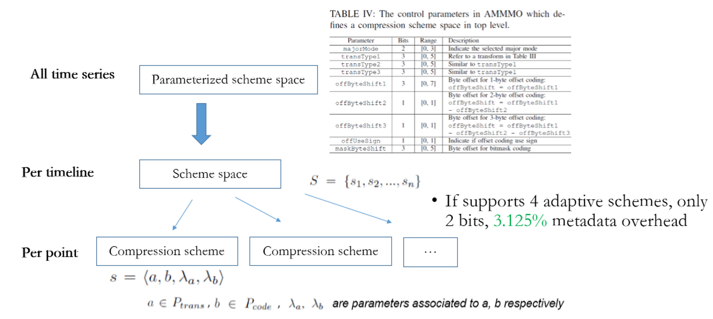
3.3 Two-Stage Compression Framework: AMMMO

The overall process of adaptive multiple mode middle-out (AMMMO) is divided into two stages. At the first stage, determine the general characteristics of the current timeline and determine the values of nine control parameters. Then at the second stage, traverse a small number of compression patterns and select the best pattern for compression.

It is easy to choose a pattern at the second stage. However, it is challenging to obtain a proper compression space by determining the parameter values (nine values in this example) at the first stage, because a proper compression space must be selected from 300,000 combinations (in theory.)

3.4 Rule-Based Pattern and Space Selection Algorithms

We can design an algorithm that creates a scoreboard for all compression patterns. Then, the algorithm traverses all points in a timeline and performs analysis and recording. Eventually, the algorithm can select the best pattern through statistics, analysis, and comparison. Here, this process involves some obvious problems:

Selected evaluation metrics may be inappropriate.
In this problem, we must think and manually compile programs and deal with many workloads, including implementation, debugging, and maintenance.
If primitives and compression patterns of an algorithm are changed, all the code must be restructured. In addition, given that the preceding selections are not theoretically deduced, an automatic and intelligent method is required to support constant evolution.

4. Deep Reinforcement Learning

4.1 Problem Modeling

We can simplify the preceding pattern and space selection algorithm into the structure shown in the following diagram. In this way, we can consider the problem as a classification problem with multiple targets. Each parameter is a target, and the value range of each parameter space includes the available classes. Deep learning has proved its high availability in terms of image classification and semantics understanding. Similarly, we can also implement the pattern and space selection by using deep learning as a multi-label classification process.

Then, what kind of network can we use? Since the main relations identified include delta/xor, shift, and bitmask, the Convolutional Neural Network (CNN) is not proper, and full-connect multilayer perceptron (MLP) is proper. Take all points in a timeline into account. There are a total of 3600 x 8B points in one hour, which is a huge number. Considering the similar segments in the same timeline, we can consider 32 points as the basic processing unit.

Next, how can we create training samples and how can we determine labels for samples?

We introduced reinforcement learning instead of supervised learning for training for the following reasons.

It is difficult to create labeled samples: The size of 32 samples is 256 bytes. Theoretically, there are 256^256 possibilities for the samples. For each of these samples, we need to traverse 300 thousand possibilities to find the best one. As a result, we must deal with huge workloads for creating and selecting samples, and creating labels.
This is not a common one-class-label problem. When a sample is given, there is not only one best result. Instead, many choices may achieve the same compression effect. Accordingly, the training of N classes (N is unknown) can be more difficult.
To address this, we need an automatic method. The selection of parameters, such as the compression tool, is likely to be extended. If so, the entire training sample must be created again. Therefore, an automatic method is required for this case.

Then, which type of reinforcement learning should we select; DQN, Policy Gradient, or Actor-Critic? As we analyzed earlier, DQN does not apply to the case where rewards and actions are discontinuous. The parameters, such as majorMode 0 and 1, lead to completely different results. Therefore, DQN does not apply. In addition, it is not easy to evaluate compression problems and the network is not complex. Therefore, Actor-Critic is not required. So, we chose Policy Gradient.

A common loss of Policy Gradient is to use a slowly raised baseline as the metric for showing whether the current action is reasonable. For this sample, Policy Gradient is not suitable, with poor effects achieved. This is because the sample has too many (256^256) theoretical block states. Therefore, we designed a loss.

After we obtained the parameters of each block, we need to consider the correlation between the blocks. We can use statistical aggregation to obtain the final parameter settings of the entire timeline.

4.2 Network Framework of Deep Reinforcement Learning

The following figure shows the entire network framework.

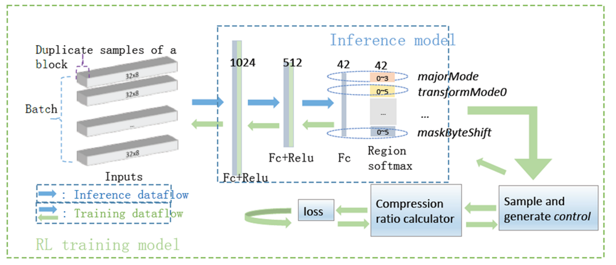
On the training side, M blocks are randomly selected, each block is copied in N duplicates, and then the duplicates are input into a fully connected network with three hidden layers. Region softmax is used to obtain the probabilities of various choices of each parameter. Then, the value of each parameter is sampled based on the probabilities. The resulting parameter values are then passed into the underlying compression algorithm for compression. Finally, a compression value is obtained. The N duplicate blocks are compared to calculate the loss and then backpropagation is performed. The overall design of the loss is:

fn(copi) describes the compression effect, which indicates positive feedback if it is higher than the average value of the N blocks. Hcs(copi) indicates the cross-entropy; the higher the probability of obtaining a high score, the more certain, and better the result, and vice versa. H(cop) indicates the cross-entropy that is used as a normalization factor to avoid network curing and perform convergence to achieve local optimum.

On the inference side, all or partial blocks of a timeline can be input into the network to obtain parameter values, which can be used for statistical aggregation to obtain the parameter values of the timeline.

5. Result Data

5.1 Experimental Design

We obtained the test data by randomly selecting a total of 28 timelines from 2 large scenarios, Alibaba Cloud IoT and the server. We also selected the data set UCR, which is the most common in the field of time series data analysis and mining. The basic information is:

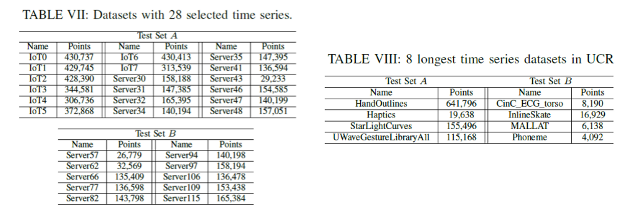
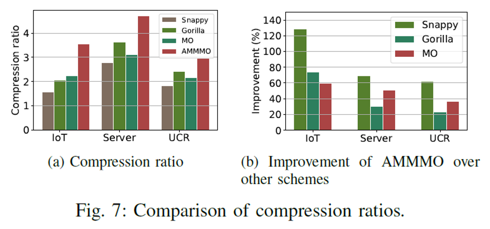
We selected Gorilla, MO, and Snappy as the comparison algorithms. Since AMMMO is a two-stage compression algorithm framework and various algorithms can be used for parameter selection at the first stage, we selected Lazy (simply setting some universal parameters), rnd1000Avg (obtaining the average effect from 1,000 random samples), Analyze (using manual code), and ML (an algorithm of deep reinforcement learning.)

5.2 Comparison of Compression Effects

In terms of the overall compression ratio, the two-stage adaptive multi-mode compression ratio of AMMMO significantly improved the compression effect, as compared with those of Gorila and MO, with the average compression ratio increases by about 50%.

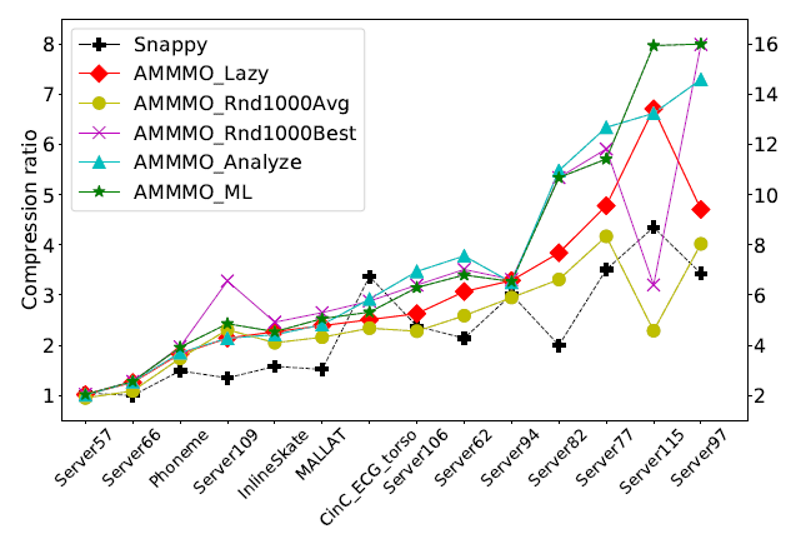
Then, what about the performance of ML? The following figure compares the compression effects on test set B in terms of ML. In general, ML is slightly better than Analyze and much better than rnd1000Avg.

5.3 Running Efficiency

Based on the design concept of MO, AMMMO removed bit-packing. This allows AMMMO to run at high speeds on CPUs. It also makes it ideal for parallel computing platforms, such as GPUs. In addition, AMMMO is divided into two stages. The first stage has poorer performance, but most of the time, the global compression parameters can be reused. For example, the data of a specific device from the last two days is reusable. The following figure shows the overall performance comparison. The experimental environment is "Intel CPU 8163 + Nvidia GPU P100" and the AMMMO code is P100.

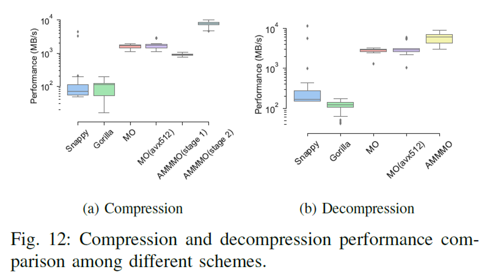
As shown in the preceding figure, AMMMO achieved the Gbit/s-level processing performance on both the compression and decompression ends, and the values of performance metrics are good.

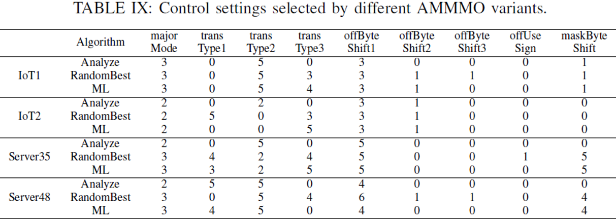
5.4 The Effect of Algorithm Learning

The network trained by deep reinforcement learning achieved a good final effect. So, did it learn meaningful content? The following table compares the performance of the three algorithms on several test sets. We can see that the parameter selection of ML is similar to those of Analyze and RandomBest, especially in the selection of byte offset and majorMode.

So, what is the representation of the compressed full-connect network parameters? We visualized the parameter heatmap at the first layer, as shown in the following figure. Positive parameter values are displayed in red, and negative parameter values are in blue; the larger the values, the brighter the color.

We can see that the values of 32 points are regularly displayed in vertical lines within the same bytes. Obfuscation occurs across bytes, and we can consider delta or xor computing occurs at the corresponding positions. The parameters of Byte0 with the largest number change are also active.

The views expressed herein are for reference only and don't necessarily represent the official views of Alibaba Cloud.

Community

Application of Deep Reinforcement Learning in Time Series Data Compression - ICDE 2020 Paper

Acknowledgment of the People Involved

Preface

1. Background

1.1 Time Series Data

1.2 Reinforcement Learning

2. Compression of Time Series Data

3. Two-Stage Compression Algorithms Based on Deep Learning

3.1 Characteristics of Time Series Data Compression

3.2 Core Concepts of New Algorithms

3.3 Two-Stage Compression Framework: AMMMO

3.4 Rule-Based Pattern and Space Selection Algorithms

4. Deep Reinforcement Learning

4.1 Problem Modeling

4.2 Network Framework of Deep Reinforcement Learning

5. Result Data

5.1 Experimental Design

5.2 Comparison of Compression Effects

5.3 Running Efficiency

5.4 The Effect of Algorithm Learning

Read previous post:

Read next post:

Alibaba Clouder

You may also like

Comments

Alibaba Clouder

Related Products

Platform For AI

AIRec

Artificial Intelligence Service for Conversational Chatbots Solution

Epidemic Prediction Solution